Some Notes on Decision Trees

Entropy

The concept of entropy was developed by the physicist Ludwig Boltzmann in the late 19th century. It is one of the most mysterious concepts in all of physics. The entropy concept was developed from the study of thermodynamic systems, in particular statistical mechanics. The entropy law is sometimes refered to as the sceond law of thermodynamics. (The first law of thermodynamics is the law of conservation of energy.)

This second law states that for any irreversible process, entropy always increases. Entropy is a measure of disorder. So the second law states that any irreversible process, the disorder in the universe increases.


	For a simple example of an irreversible process say you have a bottle of ink and a bottle of water. Pour the ink into the water. Now try to separate the two liquids.

Since virtually all natural processes are irreversble, the entropy law implies that the universe is "running down". Order, patterns, structure, all gradually disintegrate into random disorder. The entropy law therefore defines the direction of time itself, the direction from order to chaos. "Time flies like an arrow", and the direction of the arrow of time is into chaos. Physicists refer to the "heat death" of the universe.

Boltzmann himself committed suicide because of the depressing nature of his discovery, or so the story goes.

Entropy and Energy

On the practical side, entropy can be seen as a measure of the quality of energy. Low entropy sources of energy are of high quality. Such energy sources have a high energy density. High entropy sources of energy are closer to randomness and are therefore less available for use. For example, gasoline is high quality (low entropy), whereas wood is lower quality. You don't have wood burning aircraft.

Entropy and Information

Claude Shannon transferred some of these ideas to the world of information processing. Information is associated by him with low entropy. Contrasted with information is "noise", randomness, high entropy. Raw data may contain much information but it can be masked by real or apparent randomness, by noise, making the information unusable.

At the extreme of no information are random numbers. A collection of random numbers has no structure. It contains no patterns of any kind. It is completely unorganized. A collection of random numbers has maximum entropy: "information death".

Of course, data may only look random. There may be hidden patterns, information in the data. The whole point of data mining is to dig out the patterns. The mined patterns are usually presented as rules or decision trees. Shannon's information theory can be used to construct decision trees.

Using Information Theory in the Construction of Decision Trees

A Weka J48 Decision Tree

How it works

First just assume that we have an information caluclator at our disposal. In the next section we see how this calculator works.

The example is based on the weather data used several times before.

In real data mining situations, the problem is that the decison tree constucted may become gigantic. So it becomes important to find techniques to minimize the size of the tree, as far as possible.

The idea is to put the decision nodes which give the most information highest (closest to the root) in the decision tree.

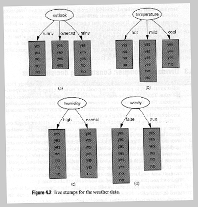
The diagram shows the four possible choices for root node in the weather example. Also shown are the numbers of yes and no classifications corresponding to each choice provided at each node.

Now consider two extremes. You could have 50% yes, and 50% no on a branch (doesn't actually happen in this example). This is the worst case. You might as well flip a coin on such a branch. There is no real information. Randomness reigns. Entropy is highest.

The other extreme is a case where 100% of the outcomes are in one class, a pure case. An example of this is shown above in the outlook->overcast branch. In this case we have certainty. Entropy is zero, information is maximal.

Of course, it may not be overcast, so the fact that that condition, if it exists, makes the choice easy because so much information is provided, we still must average in the other possibilities in some way before choosing "outlook" as our top (root) node.

In Shannon's information theory, informaion is measured in bits. These bits are not quite like computer bits because their values can range from 0 to 1 instead of just being 0 or 1.

Calculation of weighted average information for the outlook node.

info([2,3], [4,0],[3,2]) = (5/14) * 0.971 + (4/14) * 0.0 + (5/14) * 0.971 = 0.693 bits

How is this calculation interpreted?

First, note the notation: [2,3] means 2 yess and 3 no in the first branch, for example.

The value 0.971 is calculated as shown below.

The resutt, 0.693, represents the average amount of information necessary to specify the class of a new example presented to a decision tree structured as diagram (a) above.

This value must be put in a base context. How much information is needed to determine the class of an example instance starting from scratch, that is, without any decision tree at all? We have 14 examples, 9 of which are class "yes" and only 5 of which are of class "no". So we could just guess "yes" and be done with it! At least the odds are better than 50-50.

What does information theory have to say about this? The calculation for the base situation gives,

info([9,5]) = 0.940 bits.

This is the information necessary to classify an example instance without any aids such as a decision tree.

You can see that even the one level tree in diagram (a) is of some use. Without the tree we need 0.940 bits of information. With the (one node) tree in diagram (a) we only need 0.693 bits of information to classify an example.

By putting the outlook node as the root of the decision tree we have gained 0.940 - 0.693 = 0.247 bits of information.

gain(outlook) = 0.247 bits

The question then arises, is that the best we can do? We have 3 other choices for root node. It turns out that having "outlook" as root does give us the best bang for the buck. The information gains choosing the other nodes as root are,

gain(temperature) = 0.029 bits
gain(humidity) = 0.152 bits
gain(windy) = 0.048 bits

So "outlook" is the right choice if we hope to construct the smallest possible decision tree.

Recursion!

Having chosen "outlook" as the root we recursively apply the same procedure on its possible chlld nodes.

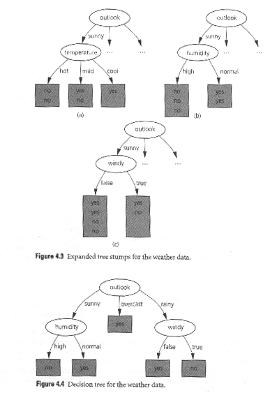
Figure 4.3 illustrates the possibilities. The information gains for each of the three cases are,

gain(temperature) = 0.571 bits
gain(humidity) = 0.971 bits
gain(windy) = 0.020 bits

The "humidty" node is the clear winner, so we split on it. This split leads to pure leaf nodes so we need no more information to decide the class of a example instance which follows these paths. The recursion bottoms out at pure leaf nodes.

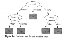
Of course, the other branches have to be analysed too. The resulting decision tree is shown in figure 4.4 above.

Calculating Information

The mysterious numbers appearing above are calulated from a formula relating information to entropy.

A measure of information needed at a decision tree node must satisfy three properties. These properties can be stated in terms of the weather example classifications. (These results are easily generalized.)

If the number of either yeses or nos is zero (the branch is pure) , the information needed is 0.
If the number of yeses equals the number of nos, then the information needed reaches a maximum.
Information must obey the "multistage property".

The first two of these properties have already been discussed.

The mulitstage property

Decisions can be made all at once or in stages. The overall information needed in each case is the same.

Example

Suppose you have a classifier with 3 classes. A certain decision tree node split points to 2 cases of the first class, 3 or the second class, and 4 of the 3rd class. Then we could write,

info([2,3,4]).

This involves one decsion.

But instead you could view things this way. Combine classes 2 and 3 which have 7 items together. Then the information for the decision would be,

info([2,7]).

Following this, it might still be necessary to decide between class 2 and class 3 if the first decision did no result in chooseing class 1. The information needed for this second decision would be

info([3,4]).

The information needed in both types of decision process is the same so,

info([2,3,4]) = info([2,7]) + (7/9) * info([3,4])

This is the multistage property of decision trees. Note the factor 7/9 which takes into account that in the two-decision case, the second decision is not always necessary.

Entropy Again

It turns out that only one function statisfies the three properties stated above - the entropy functions (sometimes called the information function). This function was originally invented by Boltzmann in the 19th century!

entropy(p₁, p₂, .... p_n) = -p₁ log p₁ - p₂ log p₂ ... - p_n log p_n

Here the logs are base 2. The p's are in the range 0 to 1. The negative signs give a positive result since the logs of fractions are also negative. The p's are related to probabilites. They represent the fractional number of states corresponding to a certain classificatioin. Therefore, the sum of the p's is 1.

info([2,3,4]) = entropy(2/9, 3/9, 4/9) = - 2/9 * log (2/9) - 3/9 * log(3/9) - 4/9 * log(4/9)

= (-2 * (log 2 - log 9) - 3 * (log 3 - log 9) - 4 * (log 4 - log 9)) / 9

Most calculators do not have base 2 logs. You can calculate them from base 10 logs using the formula,

log₂a = log₁₀a / 0.301

= (-2 * log 2 -3 log 3 -4 log4 + 9 log 9) / 9

= (-2 * 1 - 3 * 1.585 - 4 * 2 + 9 * 3.179) /9

= 1.5 bits.

Calculating the two stage decision produces the same result.

info([2,3,4]) = info([2,7]) + (7/9) * info([3,4]).

Test this:

info([2,7]) = entropy(2/9, 7/9) = - 2/9 log 2/9 - 7/9 log 7/9

= (-2 log 2 - 7 log 7 + 9 log 9) / 9 = (-2 - 19.67 + 28.13) / 9

= 0.718 bits.

info([3,4]) = entropy(3/7, 4/7)

= (-3 log 3 - 4 log 4 + 7 log 7) / 7

= (-4.755 - 8 + 19.65) / 7

= 0.985 bits.

Total info is 0.716 + (7/9) * 0.985

= 1.5 bits.

(There are round off errors in the two calculations which limit the agreement to 2 significant figures in this example :-) ).

Some "famous" decision tree machine learners

The simple algorithm described above is called ID3 and was invented by Ross Quinlan. The original simple algorithm described above has an unfortunate bias in favour of nodes with larger branching ratios. This problem can be overcome fairly easily.

Other problems include missing or noisy data. These too have been dealt with. One of the most successful decision tree generators is called C4.5. The Weka system implements a still more advanced version called J48.

Decision tree created by J48 from German credit data

Using a Decision Tree

Once a decision tree is created by a machine learning algorithm it can be used by either a human analyst or a computer program. Given a new data record, one just uses it to trace a path down the tree from the root to a leaf node containing the desired decision.

For illustration, consider the decision tree derived from the weather data and a new piece of weather information. Should the game be played or not?

outlook	temperature	humidity	windy	play
sunny	cool	high	true	?

outlook	temperature	humidity	windy	play
sunny	cool	high	true	?

Following the sunny arc from the outlook node we come to the humidity node. We follow the humidity high arc to the leaf which says no. So the decision is not to play. Apparently we did not need the temperature and windiness information to make this decision!

Decision Trees and Rules

It is easy to convert decision trees into a rule set by following all possible paths through the decision tree. For illustration, consider, once again, the weather decision tree.

IF outlook = sunny AND humidity = high THEN play = no.
IF outlook = sunny AND humidity = normal THEN play = yes.
IF outlook = overcast THEN play = yes.
IF outlook = rainy AND windy = false THEN play = yes.
IF outlook = rainy AND windy = true THEN play = no.