| home > information/tutorial > genetic algorithms | |
|
| |
|
this page navigation
| ||||||||||||||||||||||||||||
Genetic Algorithms
Introduction
The idea behind GA´s is to extract optimization strategies nature uses successfully - known as Darwinian Evolution - and transform them for application in mathematical optimization theory to find the global optimum in a defined phase space.
One could imagine a population of individual "explorers" sent into the optimization phase-space. Each explorer is defined by its genes, what means, its position inside the phase-space is coded in his genes. Every explorer has the duty to find a value of the quality of his position in the phase space. (Consider the phase-space being a number of variables in some technological process, the value of quality of any position in the phase space - in other words: any set of the variables - can be expressed by the yield of the desired chemical product.) Then the struggle of "life" begins. The three fundamental principles are
Only explorers (= genes) sitting on the best places will reproduce and create a new population. This is performed in the second step (Mating/Crossover). The "hope" behind this part of the algorithm is, that "good" sections of two parents will be recombined to yet better fitting children. In fact, many of the created children will not be successful (as in biological evolution), but a few children will indeed fulfill this hope. These "good" sections are named in some publications as building blocks.
Now there appears a problem. Repeating these steps, no new area would be explored. The two former steps would only exploit the already known regions in the phase space, which could lead to premature convergence of the algorithm with the consequence of missing the global optimum by exploiting some local optimum. The third step - the Mutation ensures the necessary accidental effects. One can imagine the new population being mixed up a little bit to bring some new information into this set of genes. Off course this has to happen in a well-balanced way!
Whereas in biology a gene is described as a macro-molecule with four different bases to code the genetic information, a gene in genetic algorithms is usually defined as a bitstring (a sequence of b 1´s and 0´s).
Remember: Don´t project results obtained from GA-performance or different qualities of algorithm types to biological/genetic procedures. The aim of GA´s is not to model genetics or biological evolution! Consider GA´s as a kind of bionic in trying to extract successful natural strategies for mathematical problems.
Back to Contents
Algorithm

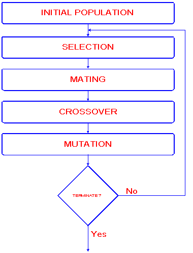
Fig.1. Schematic diagram of the algorithm
Initial Population
As described above, a gene is a string of bits. The initial population of genes (bitstrings) is usually created randomly. The length of the bitstring is depending on the problem to be solved (see section Applications).
Selection
Selection means to extract a subset of genes from an existing (in the first step, from the initial -) population, according to any definition of quality. In fact, every gene must have a meaning, so one can derive any kind of a quality measurement from it - a "value". Following this quality "value" (fitness), Selection can be performed e.g. by Selection proportional to fitness:
-
Consider the population being rated, that means: each gene has a related fitness. (How to obtain this fitness will be explained in the Application-section. ) The higher the value of the fitness, the better.
-
The mean-fitness of the population will be calculated.
-
Every individuum (=gene) will be copied as often to the new population, the better it fitness is, compared to the average fitness. E.g.: the average fitness is 5.76, the fitness of one individuum is 20.21. This individuum will be copied 3 times. All genes with a fitness at the average and below will be removed.
-
Following this steps, one can prove, that in many cases the new population will be a little smaller, than the old one. So the new population will be filled up with randomly chosen individua from the old population to the size of the old one.
Remember, that there are a lot of different implementations of these algorithms. For example the Selection module is not always creating constant population sizes. In some implementations the size of the population in dynamic. Furthermore, there exist a lot of other types of selection algorithms (the most important ones are: Proportional Fitness, Binary Tournament, Rank Based). I restrict myself to describe just the most common implementations in this short article. To get a deeper insight to this topic take a look to the Recommended Reading section.
Mating/Crossover

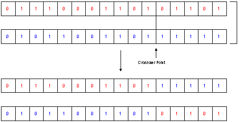
Fig.2. Crossover
The next steps in creating a new population are the Mating and Crossover: As described in the previous section there exist also a lot of different types of Mating/Crossover. One easy to understand type is the random mating with a defined probability and the b_nX crossover type. This type is described most often, as the parallel to the Crossing Over in genetics is evident:
-
PM percent of the individua of the new population will be selected randomly and mated in pairs.
-
A crossover point (see fig.2) will be chosen for each pair
-
The information after the crossover-point will be exchanged between the two individua of each pair.
In fact, more often a slightly different algorithm called b_uX is used. This crossover type usually offers higher performance in the search.
-
PM percent of the individua of the new population will be selected randomly and mated in pairs.
-
With the probability PC, two bits in the same position will be exchanged between the two individua. Thus not only one crossover point is chosen, but each bit has a certain probability to get exchanged with its counterpart in the other gene. (This is called the uniform operator)
Mutation

Fig.3. Mutation
The last step is the Mutation, with the sense of adding some effect of exploration of the phase-space to the algorithm. The implementation of Mutation is - compared to the other modules - fairly trivial: Each bit in every gene has a defined Probability P to get inverted.
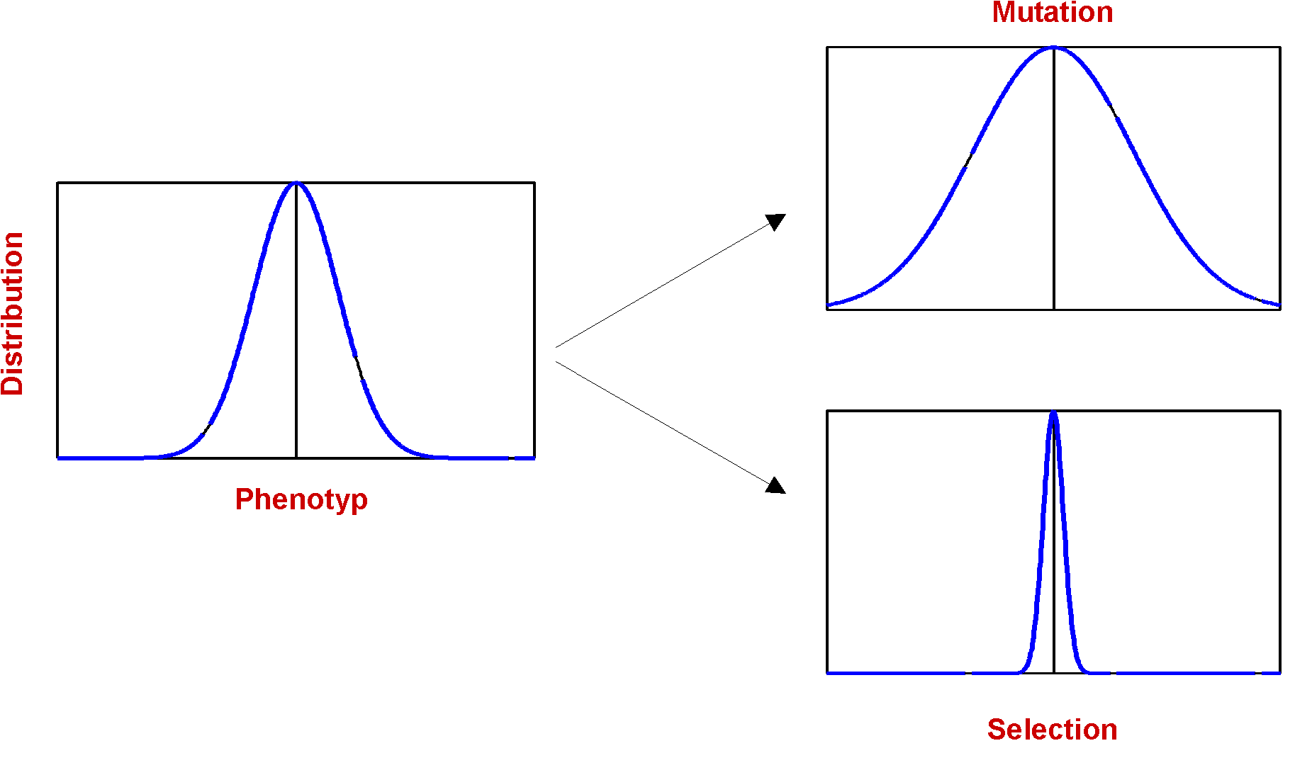
The effect of mutation is in some way a antagonist to selection:

Fig.4. Distribution of Phenotyp and the Influence of Selection and Mutation
Back to Contents
Application(s) - Coding Problems
Three important applications will be mentioned here:
Though it is impossible to explain these three categories in detail, especially implementation of Subset Selection and Sequencing shows much more traps than the Parameter Estimation problem. For better understanding of this topic, I will describe the Parameter Estimation in more details. The other two points are well explained in Lucasius et.al.
Parameter Estimation
Consider a statistical model f(x1, x2, ... xi) with parameters (a1, a2, ... aj ) and the data set (y1, y2, ... yk ). The task is to calculate the estimated parameters (a'1, a'2, ... a'j ).
In many cases the calculation of the estimated parameters is possible with an mathematically derived formula (see Linear Regression). But in many interesting instances this is not possible. Furthermore, every time varying the model, a new derivation of the solution is necessary. Using GA´s can be a good solution in these (often rather complex) problems.

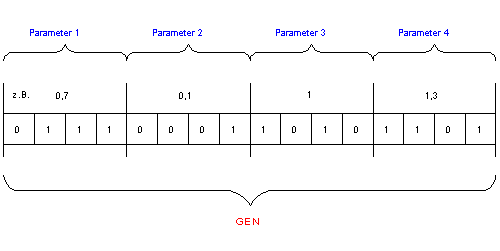
Fig.4.: Example for Parameter Transformation from real - variables to the GA-bitstring
How to solve the problem, that the model is described by a set of (usually) real - type variables, but genetic algorithms work with a bitstring as phase-space representation?
The usual way is (example see fig.4):
-
Scale the variables to integer variable by multiplying them with 10n, where n is the number of comma-places ( the desired precision):
New Variable = integer(Old Variable ×10 n)
-
Transform the variables to binary form
-
Connect all binary representations of these variables to the desired bitstring.
-
If the sign is necessary two ways are possible:
-
Add the lowest allows value to the variable and transform the variables to positive ones
-
Reserve one bit per variable for the sign
-
Remark: Usually not the binary representation is used, but the Gray-code representation (see Vankeerberghen et.al.)
How to use the algorithm?
-
Define the bitstring with the necessary length (see explanation of the coding above)
-
Make random initial - population
-
start genetic algorithm as shown in fig.1
-
after the mutation step: transform the bitstring of each individuum back to the model-variables
-
test the quality of fit for each parameter set (= individuum) (e.g. using the sum of squared residuals; as the quality of fit has to be increasing with better quality, take 1 / LS as value for the fitness)
-
check if quality of the best individuum is good enough, if so: stop iteration, otherwise restart algorithm: do selection, mating, crossover, mutation, calculate fitness, ...
Remark: As it is not easily possible to define a threshold of fitness to stop iteration (as the search-space is not known in detail) in many cases, often a defined number of iterations (= generations) is calculated. It is advisable to perform more than one GA-calculation of one fit to increase the probability, that the GA - had found the global optimum.
In a more general way, the problem could be described as
follows: Imagine a black-box with n - knobs, and one
display in front of it, that shows a value (= a
fitness!). The position of the knobs is correlated in some way
with the value shown in the display (but not necessarily described in
detail!). The duty is to turn these knobs with a good
strategy to find the position showing the highest (or
equivalently the lowest) value in the display. This good strategy
can be using a genetic algorithm.
So - in general - every
problem one can formulate in this
"black-box" way, giving a
response to a set of variables
(or a bitstring) can be optimized (solved) using a genetic algorithm!
Subset Selection
Consider a set of items (e.g. lots of data acquired with a multi-sensor array, spectroscopical data as IR- or MS - spectra, ...). Reducing the size of the dataset by extracting a subset, containing the essential information for some application (recognition of functional groups, detection of pesticides) is called a Subset Selection problem.
Two ways of coding a Subset Selection problem are common:
-
Each set n-th bit of the bitstring represents the existence of the datapoint n in the subset (E.g. {01010110} means that datapoint 2, 4, 6 and 7 are in the selected subset)
-
The size of the subset has a defined size of m datapoint:
-
the bitstring is built of m variables
-
each variable represents a number of the datapoint n being in the subset. (the example above, each variable is coded with 3 bits: the bitstring {001 011 101 111}means that datapoint 1, 3, 5 and 7 are in the selected subset)
-
More details of implementation are described in Lucasius et.al..
Sequencing
Finding an good or optimal order of a given set of items is called a sequencing problem (E.g. Traveling Salesman problems, finding optimal order of chromatographic columns, ...). A representation of the problem could be a permutation of numerical elements (e.g. 4 3 6 1 2 5). A problem in implementation is, that (as in some representations of Subset Selection problems) each element has to occur precisely once!
Back to Contents
Recommended Reading
Books
-
Goldberg, D.E., Genetic Algorithms in Search Optimization and Machine Learning, Addison Wesley Publishing Co.Inc: Reading, MA, 1989
-
Schöneburg E., Heinzmann F., Feddersen S., Genetische Algorithmen und Evolutionsstrategien, Addison Wesley ISBN 3-89319-493-2, 1994
Articles
-
Holland J.H., Genetic Algorithms, Scientific American July 1992 (p.44-50)
-
Vankeerberghen P., Smeyers-Verbeke J., Leardi R., Karr C.L., Massart D.L., Robust Regression and Outlier Detection for non-linear Models using Genetic Algorithms, Chemometrics and Intelligent Laboratory Systems 28 (1995) 73-87
-
Lucasius C.B., Kateman G., Understanding and Using Genetic Algorithms, Part 1. Concepts, Properties and Context, Chemometrics and Intelligent Laboratory Systems, 19 (1993) pp.1-33
-
Lucasius C.B., Kateman G., Understanding and Using Genetic Algorithms, Part 2. Representation, configuration and hybridization, Chemometrics and Intelligent Laboratory Systems 25 (1994) 99-145
Back to Contents
Contact the Author
This is one of the first versions of this introduction to Genetic Algorithms. If you have further questions, recommendations or complaints - or maybe some of you would like to contribute some topics - however, any response is welcome, please send me an email.
I would be glad hearing from you if you liked this introduction or if you think something is missing or even wrong! If someone likes to use this document for some purpose or likes to mirror it on his/her homepage, let´s talk about it.
best regards
Alexander Schatten
Back to Contents
|
| |
| top | last modification 19.06.2002 22:09 |