Quadratic Eigenproblem
ALBEpack can easily be used to solve the quadratic eigenproblem. The problem has the following form
( lambda^2 M + lambda C + K ) x = 0
where M, C, and K are matrices, lambda is an eigenvalue, and x a corresponding
right eigenvector.
To solve the quadratic eigenproblem, first give it the following generalized eigenvalue problem form, by linearizing.
A z = lambda B z
Vector z is a right eigenvector.
The matrices A and B are constructed in the following manner.
                  --    --                --    --
                  | 0  I |                | I  0 |
            A  =  |      |          B  =  |      |
                  |-K -C |                | 0  M |
                  --    --                --    --
This linearization is detailed in Templates for the Solution of
Algebraic Eigenvalue Problems, section 9.2.2.
MAKE LINK
Once the problem is stated in this form, it can be given to ABLEpack's
ppp function, with the problem parameter set to 2. Please note that A could easily be singular. If it is, do not use a shift value alpha of zero.
Once the linear problem is solved by ppp, the approximate eigenvalues are stored in the ritz array. The approximate eigenvectors need some postprocessing. Let z be a right eigenvector of the linear problem, and w be a left eigenvector. They are related to the quadratic right eigenvector x and left eigenvector y like so:
              --        --             --                   --
              |     x    |             | ( lambda M + C )' y |
        z  =  |          |       w  =  |                     |
              | lambda x |             |          y          |
              --        --             --                   --
The example script quad_eig.m
demonstrates this use of ABLEpack.
Briefly, the script does the following:
- load matrices M, C, K
- specify shift value alpha, to be used in linear problem
- specify number of eigenvalues to find, neig
- construct matrices A and B
- initialize ppp input parameters
- call ppp
- convert linear problem eigenvectors to quadratic problem eigenvectors
- display eigenvalues and residuals
Examples
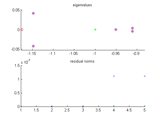
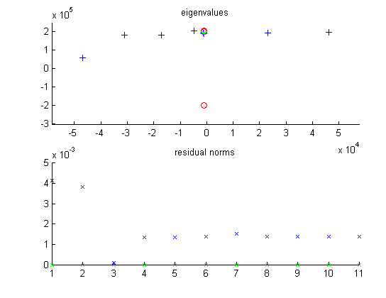
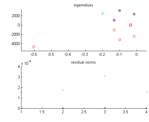
These three examples all use the quad_eig script. The desired number of eigenvalues is four. The shift value alpha is different for each problem. The figures show eigenvalues and residual norms. Approximate eigenvalues were found using ppp, while actual eigenvalues were computed by MATLAB's much more costly eig function.Mass Damper Spring System
| problem | Modal analysis of a mass / damper / spring system. |
| matrix size | 100 x 100 |
| shift value | -1.0 |
| eigenvalues desired | 4 |
| eigenvalues found | 5 |
| Lanczos steps | 22 |
In this example, M is a diagonal mass matrix, C is a diagonal damping matrix, and K is the stiffness matrix. The i'th row of matrix K has three nonzero elements. K(i,i-1) = -ki, K(i,i) = ki + ki+1, K(i,i+1) = -ki+1, where ki is the stiffness of the i'th spring. Masses, damping coefficients, and spring coefficients were random values between 0 and 1.
matrix M - mass
matrix C - damping
matrix K - spring constants
Four eigenvalues were requested, five converged. All have small residual norms, even the two largest on the order of 10e-7.

|
* shift value alpha + approximate eigenvalue, Ritz value o exact eigenvalue x right residual norm x left residual norm |
         approximate      left residual   right residual
         eigenvalues      norms           norms

         -0.95            0.00            0.00
         -0.91 -0.0042i   0.0004 e-8      0.00
         -0.91 +0.0042i   0.0004 e-8      0.00
         -1.15 -0.0419i   0.3358 e-8      0.1112 e-6
	 -1.15 +0.0419i   0.3358 e-8      0.1112 e-6
SUGAR
| problem | modal analysis of a vibrating mass electrical gap closing device |
| matrix size | 30 x 30 |
| shift value | -1000.0 + 190000i |
| eigenvalues desired | 4 |
| eigenvalues found | 11 |
| Lanczos steps | 12 |
Observe that the right residual norms are small, but the left residual norms are rather large. Only the third eigenvalue has good residual norms. Matrix A for this problem was very ill conditioned, with a condition number of 2.2342 e22. Finding a small number of approximate eigenvalues using ppp was significantly faster that finding all eigenvalues using eig.

|
* shift value alpha + approximate eigenvalue, Ritz value o exact eigenvalue x right residual norm x left residual norm |
         approximate      left residual   right residual
         eigenvalues      norms           norms

        -0.01 +1.89i e5   0.0084 e-12     0.0041
        -0.01 +1.91i e5   0.0075 e-12     0.0038
        -0.05 +2.02i e5   0.1127 e-12     0.0001   the "good" eigenvalue
         0.23 +1.91i e5   0.1799 e-12     0.0014
QEPAS
| problem | model of a bearing support shaft |
| matrix size | 80 x 80 |
| shift value | -0.2 + 2500i |
| eigenvalues desired | 4 |
| eigenvalues found | 4 |
| Lanczos steps | 15 |
All the approximate eigenvalues which are close to the actual eigenvalues, but that is due to a well chosen shift value alpha.

|
* shift value alpha + approximate eigenvalue, Ritz value o exact eigenvalue x right residual norm x left residual norm |
         approximate      left residual   right residual
         eigenvalues      norms           norms

       -0.0000 +2.37i e3  0.1528 e-3      0.00
       -0.0001 +3.14i e3  0.1757 e-3      0.00
       -0.0006 +4.68i e3  0.3133 e-3      0.3362 e-5
       -0.0001 +1.07i e3  0.1602 e-3      0.0081 e-5