Title

ECS 120 Theory of Computation
Turing machine variants
Julian Panetta
University of California, Davis

Languages recognized/decided by a Turing machine

The set of strings that \(M\) accepts is called the language recognized by \(M\), denoted \[L(M) = \{ w \in \Sigma^* \mid M \text{ accepts } w \}\]

A language \(A\) is called Turing-recognizable (or Turing-acceptable, recursively enumerable, or
computably enumerable) if some Turing machine \(M\) recognizes it (\(L(M) = A\)).

True or false: \(w \not \in L(M)\) means that Turing machine \(M\) rejects \(w\).

  • True
  • False

\(w \not \in L(M)\) means that \(M\) rejects \(w\) or loops on \(w\).

Languages Recognized/Decided by a Turing Machine

The set of strings that \(M\) accepts is called the language recognized by \(M\), denoted \[L(M) = \{ w \in \Sigma^* \mid M \text{ accepts } w \}\]

A language \(A\) is called Turing-recognizable (or Turing-acceptable, recursively enumerable, or
computably enumerable) if some Turing machine \(M\) recognizes it (\(L(M) = A\)).

Claim: Turing-recognizable languages are closed under complement because for any \(M\), we can swap the accept and reject states to form \(M'\) such that \(L(M') = \overline{L(M)}\).

  • Correct
  • Incorrect

If \(M\) loops on \(w\) then so does \(M'\).
So \(w \notin L(M)\) and \(w \notin L(M')\).
Thus \(L(M') \ne \overline{L(M)}\).

Turing-recognizable languages turn out not to be closed under complement!

Languages Recognized/Decided by a Turing Machine

The set of strings that \(M\) accepts is called the language recognized by \(M\), denoted \[L(M) = \{ w \in \Sigma^* \mid M \text{ accepts } w \}\]

A language \(A\) is called Turing-recognizable (or Turing-acceptable, recursively enumerable, or
computably enumerable) if some Turing machine \(M\) recognizes it (\(L(M) = A\)).

A language \(A\) is called co-Turing-recognizable if its complement is Turing-recognizable.
(If \(A = \overline{L(M)}\) for some Turing machine \(M\)).

  • Turing machines that loop forever on certain inputs are not helpful for solving problems!
  • A TM that halts on every input is called total.
  • A total TM \(M\) such that \(L(M) = A\) is said to decide \(A\) (\(M\) is a decider).

Languages Recognized/Decided by a Turing Machine

The set of strings that \(M\) accepts is called the language recognized by \(M\), denoted \[L(M) = \{ w \in \Sigma^* \mid M \text{ accepts } w \}\]

A language \(A\) is called Turing-recognizable (or Turing-acceptable, recursively enumerable, or
computably enumerable) if some Turing machine \(M\) recognizes it (\(L(M) = A\)).

A language \(A\) is called co-Turing-recognizable if its complement is Turing-recognizable.
(If \(A = \overline{L(M)}\) for some Turing machine \(M\)).

A language \(A\) is called Turing-decidable if there is a total Turing machine \(M\) (a decider) such that \(L(M) = A\). In other words \(M\) accepts all \(w \in A\) and rejects all \(w \notin A\).

A language is Turing-decidable if and only if it is both Turing-recognizable and co-Turing-recognizable.

Why define \(L(M)\) as the language “recognized” by \(M\) and not “decided” if deciders are more useful?
Mostly mathematical convenience/completeness: \(L(M)\) exists for all Turing machines, even if not total.

Computational power

Any CFG-decidable language is also Turing-decidable.

  • True
  • False

Proof: The simulator decides all context-free languages (using the Earley parsing algorithm.)

Computational Power Review

Any Turing-decidable language is also CFG-decidable.

  • True
  • False

Counterexample: \(\setbuild{0^n 1^n 2^n}{n \in \mathbb{N}}\)

import re
def decide(x: str) -> bool:
    return re.match(r'^0*1*2*$', x) and x.count('0') == x.count('1') == x.count('2')

Variants of Turing Machines

  • There are many different ways we could define Turing machines without changing which languages are Turing-recognizable.
  • For example, Sipser defines the tape head moves as \(\{L, R\}\) instead of \(\{L, R, S\}\).
  • We summarize this by saying the definition is robust (not sensitive to changes), explaining its ability to model anything a computer can do.
  • Let’s consider how we might relieve the apparent limitation of a single sequential tape:
    • Use multiple tapes (one for input and the other for scratch space).
    • Use a two-way infinite tape (instead of one-way infinite).
    • Use multiple tape heads on a single tape.
    • Use a “2D tape” (i.e., an unbounded grid of cells in the 2D plane), a model of “scratch paper”.
    • Use random-access memory (allow \(M\) read/write access to an auxiliary “address tape;” teleport the main tape head to addresses as they are read).
  • All of these appear more powerful than a single tape Turing machine, but aren’t.
  • How do we prove this? Simulate them on a standard TM!

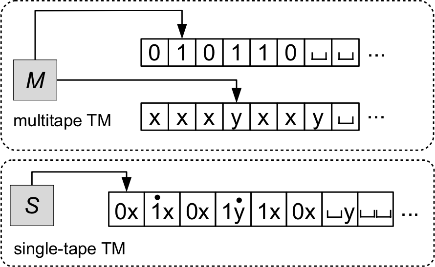
Multitape Turing Machines

data/images/tm/three_tape.svg
  • A multitape Turing machine is an ordinary Turing machine but with \(k\) tapes.
    • Each tape has its own independent read/write head.

    • The input is loaded onto the first tape, and the other tapes start blank.

    • Its transition function has the signature: \[ \delta: \fragment{(Q \setminus \{q_a, q_r\}) \times} \fragment{\Gamma^k} \to \fragment{Q} \fragment{\times \Gamma^k} \fragment{\times \{L, R, S\}^k} \]

      \[ \fragment{ \delta(q, a_1, \ldots, a_k) = (q', b_1, \ldots, b_k, m_1, \ldots, m_k) } \]

  • Theorem: For every multitape Turing machine \(M\) there is a single-tape Turing machine \(S\) such that \(L(M) = L(S)\). Furthermore if \(M\) is total, then \(S\) is total.
  • Proof idea: Construct \(S\) to simulate \(M\) on a given input.

Simulating a multitape Turing Machine

data/images/tm/three_tape.svg
  • In order to define \(S\), we have to describe how it:

    1. Encodes any configuration \(C_M\) of \(M\) as a configuration \(C_S\) of \(S\).
    2. Initially sets up its tape to simulate \(M\) (i.e., gets to the configuration encoding \(M\)’s initial configuration).
    3. Moves from \(C_S\) to a new configuration representing \(C'_M\) when \(C_M \to C'_M\).

Simulating multiple tapes: Configuration encoding

  • A configuration of \(C_M\) looks like: \[ C_M = (q, p_1, \ldots, p_k, w_1, \ldots, w_k) \]
  • We need to encode \(k\) tape head positions and \(k\) tape contents!
  • Idea: encode that a head is pointing at a character on the tape with a special marker.
    • Graphically: replace \(a \in \Gamma\) with \(\markedCharacter{a}\) (e.g., \(\markedCharacter{\string{x}}, \markedCharacter{\string{0}}, \markedCharacter{\#}\)).
    • Formally: we can represent marked/unmarked characters as tuples in \(\Gamma \cross \{\circ, \bullet\}\) (e.g., \((\string{x}, \circ)\) and \((\string{x}, \bullet)\)).
  • To encode tape contents \(w_1\), \(w_2\), \(\ldots\), \(w_k\), we have a few options:
    • Sipser’s approach: concatenate the tape contents with \(\#\) delimiters
      marking their starts and ends (assuming \(\# \notin \Gamma\)). \[ \# w_1 \# w_2 \# \cdots \# w_k \# \]
    • Our approach: form “compound symbols” to represent the characters at the same cell of each tape.
      • Graphically: a single smushed-together symbol like \(\string{b} \markedCharacter{\string{0}} \string{x}\) to represent three tapes with respective symbols \(\string{b}, \string{0}, \string{x}\).
      • Formally: an element of \((\Gamma \cross \{\circ, \bullet\})^k\)
data/images/tm/two_tape_to_one_tape.png

Simulating Multiple Tapes: Setup and Execution

data/images/tm/two_tape_to_one_tape.png
  • Given input \(x\), setup is easy in both variants.
    • Sipser: \(\# \markedCharacter{x_1} x_2 \cdots x_n \# \markedCharacter{⎵} \# \cdots \# \markedCharacter{⎵} \#\).
      1. Write \(\# \markedCharacter{x_1}\).
      2. Copy the rest of the input from \(x\) with no markers.
      3. Write \(k - 1\) copies of \(\# \markedCharacter{⎵}\), followed by a final \(\#\).
    • Ours: \(\markedCharacter{x_1}\markedCharacter{⎵}^{k - 1}\; x_2{⎵}^{k - 1} \; \cdots \; x_n{⎵}^{k - 1}\)
      • Write \(\markedCharacter{x_1}\markedCharacter{⎵}^{k - 1}\)
      • For each remaining character, write \(x_1⎵^{k - 1}\)
  • To simulate each transition:
    • Scan through the tape until all \(k\) markers are found, and remember the symbols under them.
      This is a finite amount of information: \((a_1, \cdots, a_k) \in \Gamma^k\))
    • \(M\)’s transition function can now be consulted \(\delta(q, a_1, \cdots, a_k)\).
    • Do another pass through the tape the beginning, writing the appropriate symbols around each marked character to update the character and move the marker.

Actually weaker variants

  • Move-right-or-reset: the tape head can only move right or reset to the leftmost position.
  • Two stacks
    • But using just one stack reduces the power to a deterministic pushdown automaton, incapable of deciding even certain context-free languages.
  • One queue: a.k.a., “clockwise Turing machine”… why call it that?
  • Three counters: three nonnegative integers that we can increment, decrement (if not already 0), and check if they are 0
    • But using one counter is equivalent to a unary single-stack machine, which can decide \(\setbuild{0^n 1^n}{n \in \mathbb{N}}\) but not \(\setbuild{w = \reverse{w}}{w \in \binary^*}\))
    • Even two counters are Turing universal! (under a strange encoding of the integers)