Title
Recall: Formal Definition of a Turing Machine
Recall: A Turing machine (TM) is a 7-tuple: \(M = (Q, \Sigma, \Gamma, \delta, s, q_a, q_r)\) where:

- \(Q\) is a finite set of states.
- \(\Sigma\) is a finite set of input symbols (the input alphabet).
- \(\Gamma\) is a finite set of tape symbols (the tape alphabet) with:
\(\Sigma \subsetneq \Gamma\) and blank symbol ⎵ \(\in \Gamma \setminus \Sigma\). - \(s \in Q\) is the start state.
- \(q_a \in Q\) is the accept state.
- \(q_r \in Q\) is the reject state, where \(q_r \ne q_a\).
- \(\delta: (Q \setminus \{q_a, q_r\}) \times \Gamma \to Q \times \Gamma \times \{L, R, S\}\) is the transition function
\(L\) = move left, \(R\) = move right, \(S\) = stay in place.
Formal Definition of Computation for Turing Machines
How can we describe the “full state” that a Turing machine is in (including its tape)?
A configuration of a TM \(M = (Q, \Sigma, \Gamma, \delta, s, q_a, q_r)\) is a triple: \(C = (q, p, w)\) where:
- \(q \in Q\) is the current state of the TM.
- \(p \in \N^+\) is the tape head position.
- \(w \in \Gamma^\infty\) is a one-way infinite sequence holding the tape content
Sipser uses a different notation “\(u\, q\, v\)” where \(w=uv\) and \(p = |u| + 1\).
Example: \(1011q_70111\).
See Optional Section 8.4 for a definition (uglier) using a finite, growable tape.
Formal Definition of Computation for Turing Machines
A configuration of a TM \(M = (Q, \Sigma, \Gamma, \delta, s, q_a, q_r)\) is a triple: \(C = (q, p, w)\) where:
- \(q \in Q\) is the current state of the TM.
- \(p \in \N^+\) is the tape head position.
- \(w \in \Gamma^\infty\) is a one-way infinite sequence holding the tape content
We define computation by formally specifying how one configuration \(C = (q, p, w)\) transitions to the next configuration \(C' = (q', p', w')\).
We say \(C\) yields \(C'\) (writing \(C \to C'\)) when \(M\) can legally go from \(C\) to \(C'\) in one step: \[ \delta(q, w[p]) = (\fragment{q'}, \fragment{w'[p]}, \fragment{m}) \hspace{5em} \]
We identify moves \(m \in \{L, R, S\}\) with offsets \(\{-1, +1, 0\}\) added to \(p\).
- \(p' = \max(1, p + m)\)
(Move tape head according to \(m\) but don’t go off the left end.) - \(w[i] = w'[i]\) for all \(i \ne p\)
(Leave all other tape cells unchanged.)
- \(p' = \max(1, p + m)\)
Formal Definition of Computation for Turing Machines
A configuration of a TM \(M = (Q, \Sigma, \Gamma, \delta, s, q_a, q_r)\) is a triple: \(C = (q, p, w)\) where:
- \(q \in Q\) is the current state of the TM.
- \(p \in \N^+\) is the tape head position.
- \(w \in \Gamma^\infty\) is a one-way infinite sequence holding the tape content
A configuration \((q, p, w)\) is called:
accepting if \(q = q_a\), rejecting if \(q = q_r\), halting if \(q \in \{q_a, q_r\}\).\(M\) accepts/rejects input \(w \in \Sigma^*\) if there is a finite sequence of configurations \(C_1, C_2, \ldots, C_k\) such that:
- \(C_1 = (\fragment{s}, \fragment{1}, \fragment{w \string{⎵}^\infty})\)
- \(C_i \to C_{i+1}\) for all \(1 \leq i < k\)
- \(C_k\) is accepting/rejecting
If \(M\) neither accepts nor rejects \(w\), we say \(M\) loops (does not halt) on \(w\).
- Three possible outcomes: accept, reject, or loop!
- Defining the languages “recognized” or “decided” by a TM requires more care than with FAs or CFGs.
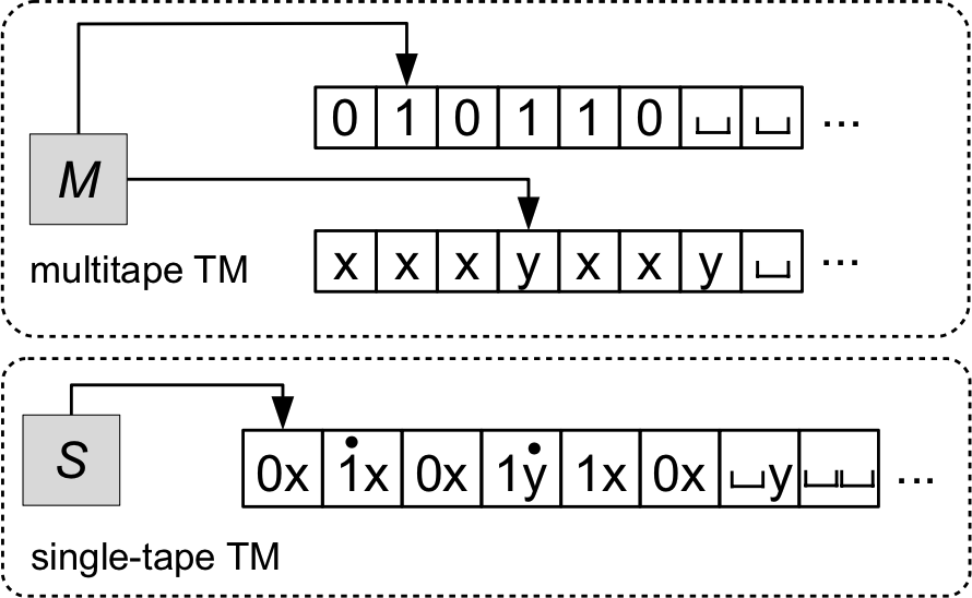
Multitape Turing Machines

- A multitape Turing machine is an ordinary Turing machine but with \(k\) tapes.
Each tape has its own independent read/write head.
The input is loaded onto the first tape, and the other tapes start blank.
Its transition function has the signature: \[ \delta: \fragment{(Q \setminus \{q_a, q_r\}) \times} \fragment{\Gamma^k} \to \fragment{Q} \fragment{\times \Gamma^k} \fragment{\times \{L, R, S\}^k} \]
\[ \fragment{ \delta(q, a_1, \ldots, a_k) = (q', b_1, \ldots, b_k, m_1, \ldots, m_k) } \]
- Theorem: For every multitape Turing machine \(M\) there is a single-tape Turing machine \(S\) such that \(L(M) = L(S)\). Furthermore if \(M\) is total, then \(S\) is total.
- Proof idea: Construct \(S\) to simulate \(M\) on a given input.
Simulating a multitape Turing Machine
In order to define \(S\), we have to describe how it:
- Encodes any configuration \(C_M\) of \(M\) as a configuration \(C_S\) of \(S\).
- Initially sets up its tape to simulate \(M\) (i.e., gets to the configuration encoding \(M\)’s initial configuration).
- Moves from \(C_S\) to a new configuration representing \(C'_M\) when \(C_M \to C'_M\).
Simulating multiple tapes: Configuration encoding
- A configuration of \(C_M\) looks like: \[ C_M = (q, p_1, \ldots, p_k, w_1, \ldots, w_k) \]
- We need to encode \(k\) tape head positions and \(k\) tape contents!
- Idea: encode that a head is pointing at a character on the tape with a special marker.
- Graphically: replace \(a \in \Gamma\) with \(\markedCharacter{a}\) (e.g., \(\markedCharacter{\string{x}}, \markedCharacter{\string{0}}, \markedCharacter{\#}\)).
- Formally: we can represent marked/unmarked characters as tuples in \(\Gamma \cross \{\circ, \bullet\}\) (e.g., \((\string{x}, \circ)\) and \((\string{x}, \bullet)\)).
- To encode tape contents \(w_1\), \(w_2\), \(\ldots\), \(w_k\), we have a few options:
- Sipser’s approach: concatenate the tape contents with \(\#\) delimiters
marking their starts and ends (assuming \(\# \notin \Gamma\)). \[ \# w_1 \# w_2 \# \cdots \# w_k \# \] - Our approach: form “compound symbols” to represent the characters at the same cell of each tape.
- Graphically: a single smushed-together symbol like \(\string{b} \markedCharacter{\string{0}} \string{x}\) to represent three tapes with respective symbols \(\string{b}, \string{0}, \string{x}\).
- Formally: an element of \((\Gamma \cross \{\circ, \bullet\})^k\)
- Sipser’s approach: concatenate the tape contents with \(\#\) delimiters
Simulating Multiple Tapes: Setup and Execution
- Given input \(x\), setup is easy in both variants.
- Sipser: \(\# \markedCharacter{x_1} x_2 \cdots x_n \# \markedCharacter{⎵} \# \cdots \# \markedCharacter{⎵} \#\).
- Write \(\# \markedCharacter{x_1}\).
- Copy the rest of the input from \(x\) with no markers.
- Write \(k - 1\) copies of \(\# \markedCharacter{⎵}\), followed by a final \(\#\).
- Ours: \(\markedCharacter{x_1}\markedCharacter{⎵}^{k - 1}\; x_2{⎵}^{k - 1} \; \cdots \; x_n{⎵}^{k - 1}\)
- Write \(\markedCharacter{x_1}\markedCharacter{⎵}^{k - 1}\)
- For each remaining character, write \(x_1⎵^{k - 1}\)
- Sipser: \(\# \markedCharacter{x_1} x_2 \cdots x_n \# \markedCharacter{⎵} \# \cdots \# \markedCharacter{⎵} \#\).
- To simulate each transition:
- Scan through the tape until all \(k\) markers are found, and remember the symbols under them.
This is a finite amount of information: \((a_1, \cdots, a_k) \in \Gamma^k\)) - \(M\)’s transition function can now be consulted \(\delta(q, a_1, \cdots, a_k)\).
- Do another pass through the tape the beginning, writing the appropriate symbols around each marked character to update the character and move the marker.
- Scan through the tape until all \(k\) markers are found, and remember the symbols under them.
Turing Machines vs. Programs
Consider the problem of comparing two strings \(x\) and \(y\) to see if they are equal.
This is trivial to do in code:
def compare(x, y):
    if len(x) != len(y):
        return False
    for i in range(len(x)):
        if x[i] != y[i]:
            return False
    return True
and it’s easy to count the number of “operations” run.
How can we do this with a Turing machine?
- Decision problem: check if \(x \# y\) is in the language \(L = \setbuild{w \# w}{w \in \Sigma^*}\).
- The Turing machine would need to:
- Zig-zag across the tape to corresponding cells on each side of the \(\#\).
- If the symbols mismatch, reject.
- If they match, cross them off by writing \(\string{x}\) symbols.
- When all symbols to the left of \(\#\) are crossed off, accept if remaining symbols are all \(\#\) or \(\string{x}\); reject otherwise.
- Zig-zag across the tape to corresponding cells on each side of the \(\#\).

Object Encoding for Turing Machines
- But programs can obviously operate on fancier objects than strings.
How can a Turing machine do this too? - For example, how can a TM read a graph?

Node and edge lists: \(\encoding{G} = \fragment{\text{(binary encoding of) } (1,2,3,4)}\fragment{((1,2),(2,3),(3,1),(1,4))}\)
We use \(\encoding{O}\) to denote the encoding of an object \(O\) as a string in \(\binary^*\). We can encode multiple objects with \(\encoding{(O_1, O_2, \ldots, O_k)}\) or just \(\encoding{O_1, O_2, \ldots, O_k}\).
Adjacency matrix: \[ \fragment{\begin{bmatrix} 0 & 1 & 1 & 1 \\ 1 & 0 & 1 & 0 \\ 1 & 1 & 0 & 0 \\ 1 & 0 & 0 & 0 \\ \end{bmatrix}} \fragment{\quad \Longrightarrow \quad \encoding{G} = } \fragment{0111101011001000} \hspace{15em} \]
How can we determine the number of nodes?
(labels don’t matter).