Title

ECS 120 Theory of Computation
Languages of Turing machines, Turing machine variants, and TMs versus code
David Doty (adapted from slides authored by Julian Panetta)
University of California, Davis

Languages recognized/decided by a Turing machine

The set of strings that \(M\) accepts is called the language recognized by \(M\), denoted \[L(M) = \{ w \in \Sigma^* \mid M \text{ accepts } w \}\]

A language \(A\) is called Turing-recognizable (or Turing-acceptable, recursively enumerable, or
computably enumerable) if some Turing machine \(M\) recognizes it (\(L(M) = A\)).

True or false: \(w \not \in L(M)\) means that Turing machine \(M\) rejects \(w\).

\(w \not \in L(M)\) means that \(M\) rejects \(w\) or loops on \(w\).

Languages recognized/decided by a Turing machine

The set of strings that \(M\) accepts is called the language recognized by \(M\), denoted \[L(M) = \{ w \in \Sigma^* \mid M \text{ accepts } w \}\]

A language \(A\) is called Turing-recognizable (or Turing-acceptable, recursively enumerable, or
computably enumerable) if some Turing machine \(M\) recognizes it (\(L(M) = A\)).

Claim: Turing-recognizable languages are closed under complement because for any \(M\), we can swap the accept and reject states to form \(M'\) such that \(L(M') = \overline{L(M)}\).

If \(M\) loops on \(w\) then so does \(M'\).
So \(w \notin L(M)\) and \(w \notin L(M')\).
Thus \(L(M') \ne \overline{L(M)}\).

Turing-recognizable languages turn out not to be closed under complement!

Languages recognized/decided by a Turing machine

The set of strings that \(M\) accepts is called the language recognized by \(M\), denoted \[L(M) = \{ w \in \Sigma^* \mid M \text{ accepts } w \}\]

A language \(A\) is called Turing-recognizable (or Turing-acceptable, recursively enumerable, or
computably enumerable) if some Turing machine \(M\) recognizes it (\(L(M) = A\)).

A language \(A\) is called co-Turing-recognizable if its complement is Turing-recognizable.
(If \(A = \overline{L(M)}\) for some Turing machine \(M\)).

  • Turing machines that loop forever on certain inputs are not helpful for solving problems!
  • A TM that halts on every input is called total.
  • A total TM \(M\) such that \(L(M) = A\) is said to decide \(A\) (\(M\) is a decider).

Languages recognized/decided by a Turing machine

The set of strings that \(M\) accepts is called the language recognized by \(M\), denoted \[L(M) = \{ w \in \Sigma^* \mid M \text{ accepts } w \}\]

A language \(A\) is called Turing-recognizable (or Turing-acceptable, recursively enumerable, or
computably enumerable) if some Turing machine \(M\) recognizes it (\(L(M) = A\)).

A language \(A\) is called co-Turing-recognizable if its complement is Turing-recognizable.
(If \(A = \overline{L(M)}\) for some Turing machine \(M\)).

A language \(A\) is called Turing-decidable if there is a total Turing machine \(M\) (a decider) such that \(L(M) = A\). In other words \(M\) accepts all \(w \in A\) and rejects all \(w \notin A\).

A language is Turing-decidable if and only if it is both Turing-recognizable and co-Turing-recognizable.

Why define \(L(M)\) as the language “recognized” by \(M\) and not “decided” if deciders are more useful?
Mostly mathematical convenience/completeness: \(L(M)\) exists for all Turing machines, even if not total.

Computational power

Any CFG-decidable language is also Turing-decidable.

Proof: The simulator decides all context-free languages (using the Earley parsing algorithm.)

Computational power review

Any Turing-decidable language is also CFG-decidable.

Counterexample: \(\setbuild{0^n 1^n 2^n}{n \in \mathbb{N}}\)

import re


def decide(x: str) -> bool:
    return re.match(r"^0*1*2*$", x) and x.count("0") == x.count("1") == x.count("2")

Variants of Turing machines

  • There are many different ways we could define Turing machines without changing which languages are Turing-recognizable.
  • For example, Sipser defines the tape head moves as \(\{L, R\}\) instead of \(\{L, R, S\}\).
  • We summarize this by saying the definition is robust (not sensitive to changes), explaining its ability to model anything a computer can do.
  • Let’s consider how we might relieve the apparent limitation of a single sequential tape:
    • Use multiple tapes (one for input and the other for scratch space).
    • Use a two-way infinite tape (instead of one-way infinite).
    • Use multiple tape heads on a single tape.
    • Use a “2D tape” (i.e., an unbounded grid of cells in the 2D plane), a model of “scratch paper”.
    • Use random-access memory (allow \(M\) read/write access to an auxiliary “address tape;” teleport the main tape head to addresses as they are read).
  • All of these appear more powerful than a single tape Turing machine, but aren’t.
  • How do we prove this? Simulate them on a standard TM!

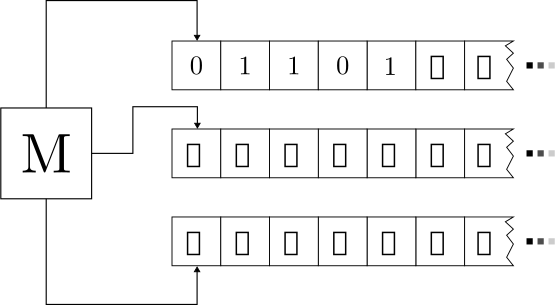
Multitape Turing machines

data/images/tm/three_tape.svg
  • A multitape Turing machine is an ordinary Turing machine but with \(k\) tapes.
    • Each tape has its own independent read/write head.

    • The input is loaded onto the first tape, and the other tapes start blank.

    • Its transition function has the signature: \[ \delta: \fragment{(Q \setminus \{q_a, q_r\}) \times} \fragment{\Gamma^k} \to \fragment{Q} \fragment{\times \Gamma^k} \fragment{\times \{L, R, S\}^k} \]

      \[ \fragment{ \delta(q, a_1, \ldots, a_k) = (q', b_1, \ldots, b_k, m_1, \ldots, m_k) } \]

  • Theorem: For every multitape Turing machine \(M\) there is a single-tape Turing machine \(S\) such that \(L(M) = L(S)\). Furthermore if \(M\) is total, then \(S\) is total.
  • Proof idea: Construct \(S\) to simulate \(M\) on a given input.

Simulating a multitape Turing machine

data/images/tm/three_tape.svg
  • In order to define \(S\), we have to describe how it:

    1. Encodes any configuration \(C_M\) of \(M\) as a configuration \(C_S\) of \(S\).
    2. Initially sets up its tape to simulate \(M\) (i.e., gets to the configuration encoding \(M\)’s initial configuration).
    3. Moves from \(C_S\) to a new configuration representing \(C'_M\) when \(C_M \to C'_M\).

Simulating multiple tapes: Configuration encoding

  • A configuration of \(C_M\) looks like: \[ C_M = (q, p_1, \ldots, p_k, w_1, \ldots, w_k) \]
  • We need to encode \(k\) tape head positions and \(k\) tape contents!
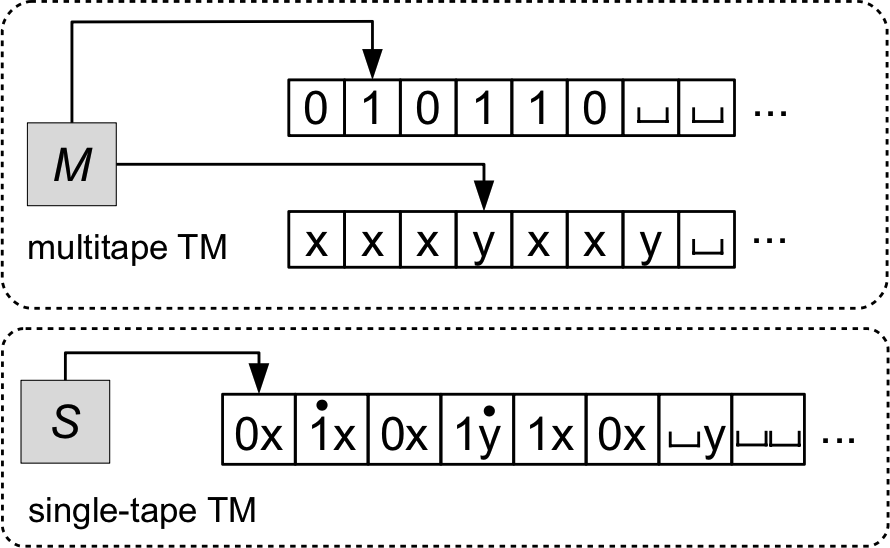
  • Idea: encode that a head is pointing at a character on the tape with a special marker.
    • Graphically: replace \(a \in \Gamma\) with \(\markedCharacter{a}\) (e.g., \(\markedCharacter{\string{x}}, \markedCharacter{\string{0}}, \markedCharacter{\#}\)).
    • Formally: we can represent marked/unmarked characters as tuples in \(\Gamma \cross \{\circ, \bullet\}\) (e.g., \((\string{x}, \circ)\) and \((\string{x}, \bullet)\)).
  • To encode tape contents \(w_1\), \(w_2\), \(\ldots\), \(w_k\), we have a few options:
    • Sipser’s approach: concatenate the tape contents with \(\#\) delimiters
      marking their starts and ends (assuming \(\# \notin \Gamma\)). \[ \# w_1 \# w_2 \# \cdots \# w_k \# \]
    • Our approach: form “compound symbols” to represent the characters at the same cell of each tape.
      • Graphically: a single smushed-together symbol like \(\string{b} \markedCharacter{\string{0}} \string{x}\) to represent three tapes with respective symbols \(\string{b}, \string{0}, \string{x}\).
      • Formally: an element of \((\Gamma \cross \{\circ, \bullet\})^k\)
data/images/tm/two_tape_to_one_tape.png

Simulating multiple tapes: Setup and execution

data/images/tm/two_tape_to_one_tape.png
  • Given input \(x\), setup is easy in both variants.
    • Sipser: \(\# \markedCharacter{x_1} x_2 \cdots x_n \# \markedCharacter{⎵} \# \cdots \# \markedCharacter{⎵} \#\).
      1. Write \(\# \markedCharacter{x_1}\).
      2. Copy the rest of the input from \(x\) with no markers.
      3. Write \(k - 1\) copies of \(\# \markedCharacter{⎵}\), followed by a final \(\#\).
    • Ours: \(\markedCharacter{x_1}\markedCharacter{⎵}^{k - 1}\; x_2{⎵}^{k - 1} \; \cdots \; x_n{⎵}^{k - 1}\)
      • Write \(\markedCharacter{x_1}\markedCharacter{⎵}^{k - 1}\)
      • For each remaining character, write \(x_1⎵^{k - 1}\)
  • To simulate each transition:
    • Scan through the tape until all \(k\) markers are found, and remember the symbols under them.
      This is a finite amount of information: \((a_1, \cdots, a_k) \in \Gamma^k\))
    • \(M\)’s transition function can now be consulted \(\delta(q, a_1, \cdots, a_k)\).
    • Do another pass through the tape the beginning, writing the appropriate symbols around each marked character to update the character and move the marker.

Actually weaker variants

  • Move-right-or-reset: the tape head can only move right or reset to the leftmost position.
  • Two stacks
    • But using just one stack reduces the power to a deterministic pushdown automaton, incapable of deciding even certain context-free languages.
  • One queue: a.k.a., “clockwise Turing machine”… why call it that?
  • Three counters: three nonnegative integers that we can increment, decrement (if not already 0), and check if they are 0
    • But using one counter is equivalent to a unary single-stack machine, which can decide \(\setbuild{0^n 1^n}{n \in \mathbb{N}}\) but not \(\setbuild{w = \reverse{w}}{w \in \binary^*}\))
    • Even two counters are Turing universal! (under a strange encoding of the integers)

Algorithms

  • Informally, an algorithm is a sequence of steps that can be followed to solve a problem.
  • Formally, we can define an algorithm as a procedure that can be implemented by a Turing machine.
  • However, after gaining some practice with Turing machines, we typically won’t specify the details of the machine.
  • Instead we can describe algorithms formally and precisely with a higher-level language (like Python).
  • We will argue that implementing a Python program on a Turing machine, while slower, won’t change its “complexity class.” (See HW3)

Object encoding for Turing machines

  • But programs can obviously operate on fancier objects than strings.
    How can a Turing machine do this too?
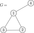
  • For example, how can a TM read a graph?
    data/images/tm/example_graph.svg
    • Node and edge lists: \(\encoding{G} = \text{(binary encoding of)}\qquad (\fragment{(1,2,3,4)}, \fragment{((1,2),(2,3),(3,1),(1,4))})\)

    • Adjacency matrix: \[ \fragment{\begin{bmatrix} 0 & 1 & 1 & 1 \\ 1 & 0 & 1 & 0 \\ 1 & 1 & 0 & 0 \\ 1 & 0 & 0 & 0 \\ \end{bmatrix}} \fragment{\quad \Longrightarrow \quad \encoding{G} = } \fragment{0111101011001000} \hspace{15em} \]

      How can we determine the number of nodes?

      We use \(\encoding{O}\) to denote the encoding of an object \(O\) as a string in \(\binary^*\). We can encode multiple objects with \(\encoding{(O_1, O_2, \ldots, O_k)}\) or just \(\encoding{O_1, O_2, \ldots, O_k}\).

Object encoding for Turing machines

  • But programs can obviously operate on fancier objects than strings.
    How can a Turing machine do this too?
  • For example, how can a TM read a graph?
  • The choice of encoding \(\encoding{\cdot}\) can matter a lot for practical reasons
    • What is the size of the adjacency matrix representation for a graph with \(n\) nodes? \(n^2\)
    • What about the node+edge list representation for a graph with \(n\) nodes and \(m\) edges?
      Proportional to \(n + m\). For sparse graphs \(m \ll n^2\)…
    • This sort of difference is a big deal, e.g., in high-performance computing.
  • But for the sorts of performance differences we study in this course, we will show any “reasonable” encoding is good enough (won’t change whether an algorithm is polynomial time or not).