Title
ECS 120 Theory of Computation
NP-Completeness and
Reductions, Pt 2
University of California,
Davis
Recall: Example Reduction to Bound Complexity of \(\probClique\)
from itertools import combinations as subsets
def reduction_from_independent_set_to_clique(G, k):
    V, E = G
    Ec = [ {u,v} for (u,v) in subsets(V,2)
            if {u,v} not in E and u!=v ]
    Gc = (V, Ec)
    return (Gc, k)
# Hypothetical polynomial-time algorithm for Independent Set
def independent_set(G, k):
    Gp, kp = reduction_from_independent_set_to_clique(G, k)
    return clique_algorithm(Gp, kp)

# Hypothetical polynomial-time algorithm for Clique
def clique_algorithm(G, k):
    raise NotImplementedError("Not implemented yet...")
- We conclude that \(\probIndSet \le^P \probClique\).
- \(\probClique\) is at least as hard as \(\probIndSet\).
- Since
reduction_from_independent_set_to_cliquealso happens to work in the other direction
(just complement again!), we can conclude also: \(\probClique \le^P \probIndSet\).
Implications of \(A \le^P B\)
Let’s now formalize what we mean by “\(B\) is at least as hard as \(A\)”
Theorem: If \(A \le^P B\) and \(B \in \P\), then \(A \in \P\).
Proof:
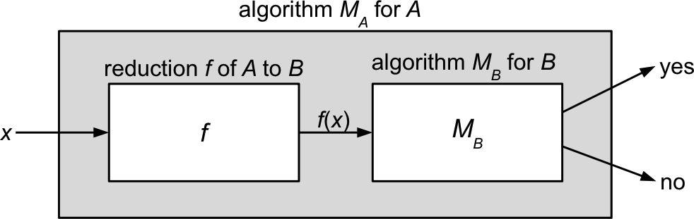
Since \(B \in \P\), there is an algorithm \(M_B\) for \(B\) that runs in time \(n^k\) for some constant \(k\)
Since \(A \le^P B\), there is a polynomial-time reduction \(f\) from \(A\) to \(B\)
(running in time \(n^c\) for some constant \(c\)).We can construct an algorithm \(M_A\) deciding \(A\) simply by composing \(f\) and \(M_B\): \[ M_A(x) = M_B(f(x)) \]
What is the time complexity of \(M_A\)? Let \(n = |x|\).
- \(O(n^c)\) for \(f(x)\), plus \(O(m^k)\) for \(M_B(f(x))\), where \(m = |f(x)|\).
- Since \(m = O(|x|^c)\), the full time complexity is: \[ O(n^c) + O(O(|x|^c)^k) \fragment{= O(n^c + n^{ck})} \fragment{= O(n^{ck})} \fragment{\quad \implies \quad A \in \P} \]