Title

ECS 120 Theory of Computation
NP-completeness, satisfiability, and polynomial-time reductions
David Doty (adapted from slides authored by Julian Panetta)
University of California, Davis

\(\NP\)-completeness

  • The practical benefit of studying \(\NP\) is being able to identify when a problem you want to solve is fundamentally “hard.”
    • Maybe you just haven’t found the right algorithm yet and should keep trying?
    • But if you can prove your problem is “at least as hard” as the hardest problems in \(\NP\), then you can be sure you’re not missing an obvious trick.
    • If \(\P \ne \NP\) (as many believe), then your problem would have no efficient solution.
  • Problems in \(\NP\) that are “at least as hard” as every other problem in \(\NP\) are called
    \(\NP\)-complete.
    • Intuitively: given an \(\NP\) complete problem \(A\), any other problem in \(\NP\) can be solved by translating it into an instance of \(A\), and then solving that.
    • This process is called a reduction from that other problem to \(A\).
  • Powerful theoretical tool: by showing a problem is \(\NP\)-complete, you show solving it for large inputs is “probably” intractable.

Example \(\NP\)-complete problem: Boolean satisfiability

  • Recall Boolean formulas: expressions involving Boolean variables and the logical operators \(\land\), \(\lor\), and \(\neg\). Example: \[ \fragment{\phi = (x \land y) \lor (z \land \neg y)} \]
  • Represent \(\TRUE\) by \(1\) and \(\FALSE\) by \(0\).
  • Operations defined by truth tables:

Negation/NOT

\[ \begin{array}{c|c} x & \neg x \\ \hline 0 & 1 \\ 1 & 0 \end{array} \]

Conjunction/AND

\[ \begin{array}{cc|c} x & y & x \land y \\ \hline 0 & 0 & 0 \\ 0 & 1 & 0 \\ 1 & 0 & 0 \\ 1 & 1 & 1 \end{array} \]

Disjunction/OR

\[ \begin{array}{cc|c} x & y & x \lor y \\ \hline 0 & 0 & 0 \\ 0 & 1 & 1 \\ 1 & 0 & 1 \\ 1 & 1 & 1 \end{array} \]

Example \(\NP\)-complete problem: Boolean satisfiability

More formally, we can define Boolean formulas inductively (like with regular expressions):

Given a finite set of variables \(V\), a Boolean formula \(\phi\) is defined as:

  • Base cases:
    1. Any \(x \in V\) is a Boolean formula.
    2. 0 and 1 are each Boolean formulas.
  • Inductive cases:
    Let \(\phi_1\) and \(\phi_2\) be Boolean formulas. Then the following are also Boolean formulas:
    1. \(\neg \phi_1\)
    2. \(\phi_1 \land \phi_2\)
    3. \(\phi_1 \lor \phi_2\)

Precedence: \(\neg\) has highest precedence, followed by \(\land\), then \(\lor\).
Parentheses can be used to override this.

We can use this recursive structure to efficiently parse and evaluate Boolean formulas.

Example \(\NP\)-complete problem: Boolean satisfiability

A Boolean formula \(\phi\) is satisfiable if there is an assignment of truth values to its variables that makes the formula evaluate to \(1\).

  • Example: \[ \phi = (x \land y) \lor (z \land \neg y) \] is satisfiable because setting \(x = 0, y = 0, z = 1\) yields \(\phi(001) = 1\).

  • We introduce the Boolean satisfiability problem:

    \[ \probSAT = \setbuild{\encoding{\phi}}{ \phi \text{ is a satisfiable Boolean formula }} \]

  • We know \(\probSAT \in \NP\) because we can easily implement a polynomial-time decider for:

    \[ \verifier{\probSAT} = \setbuild{\encoding{\phi, w}}{ \phi \text{ is a Boolean formula, and } \phi(w) = 1 } \]

    Just evaluate \(\phi\) on the assignment \(w\)!

Example \(\NP\)-complete problem: Boolean satisfiability

A Boolean formula \(\phi\) is satisfiable if there is an assignment of truth values to its variables that makes the formula evaluate to \(1\).

  • We introduce the Boolean satisfiability problem:

    \[ \probSAT = \setbuild{\encoding{\phi}}{ \phi \text{ is a satisfiable Boolean formula }} \]

  • We know \(\probSAT \in \NP\) because we can easily implement a polynomial-time decider for:

    \[ \verifier{\probSAT} = \setbuild{\encoding{\phi, w}}{ \phi \text{ is a Boolean formula, and } \phi(w) = 1 } \]

  • Cook-Levin Theorem: \(\probSAT \in \P \iff \P = \NP\).
    • In other words: we could prove \(\P = \NP\) by finding a polynomial-time algorithm for \(\probSAT\).
    • This is another way of saying \(\probSAT\) is \(\NP\)-complete.
    • \(\probSAT\) is “at least as hard” as any other problem in \(\NP\).

Reductions

  • The way you show problem \(B\) is at least as difficult as problem \(A\) is by exhibiting a reduction from \(A\) to \(B\).
    • Intuitively: we can solve an instance of \(A\) by converting it into an “equivalent” instance of \(B\).
    • Provided the conversion process is efficient, a fast algorithm for \(B\) enables an efficient algorithm for \(A\).
  • Since our notion of “efficiency” is “computable in polynomial time,” we are specifically concerned with polynomial-time reductions.

Simple reduction example: \(\probIndSet\) to \(\probClique\)

  • Recall the the \(k\)-clique problem (clique = set of nodes with edges between all pairs): \[ \probClique = \setbuild{\encoding{G, k}}{ G \text{ is an undirected graph with a } k\text{-clique}} \]

  • We now introduce a closely related problem, the \(k\)-independent set problem (independent set = set of nodes with edges between no pairs): \[ \probIndSet = \setbuild{\encoding{G, k}}{ G \text{ is an undirected graph with a } k\text{-independent set}} \]

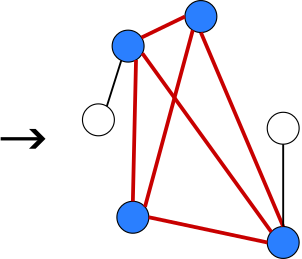
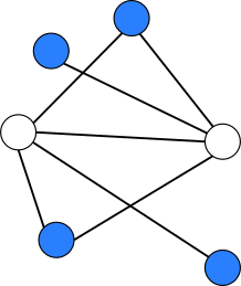
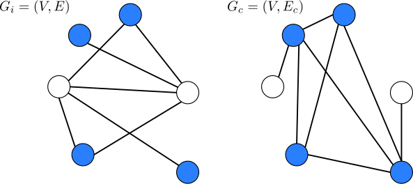
  • Given input \(\encoding{G_i, k}\) for \(\probIndSet\),
    how can we convert it to input \(\encoding{G_c, k}\) for \(\probClique\) such that:

    \[ \encoding{G_i, k} \in \probIndSet \iff \encoding{G_c, k} \in \probClique \]
    data/images/complexity/ind_set_clique_start_graph.svg
    data/images/complexity/ind_set_clique_end_graph.svg

Definition of polynomial-time reducibility

A function \(f: \binary^* \to \binary^*\) is polynomial-time computable if there is a polynomial-time algorithm that, given input \(x\), computes \(f(x)\).

Let \(A, B \subseteq \binary^*\) be decision problems. We say \(A\) is polynomial-time reducible to \(B\)
if there is a polynomial-time computable function \(f\) such that for all \(x \in \binary^*\):

\[ \fragment{x \in A \iff f(x) \in B} \]

We denote this by \(A \le^\P B\).

\(A \le^\P B\) means: “B is at least as hard as A” (to within a polynomial-time factor).

Example reduction to bound complexity of \(\probClique\)

from itertools import combinations as subsets
def reduction_from_independent_set_to_clique(G: Graph[Node], k: int) -> tuple[Graph[Node], int]:
    V, E = G
    Ec = [ {u,v} for (u,v) in subsets(V,2)
            if {u,v} not in E and u!=v ]
    Gc = (V, Ec)
    return (Gc, k)

# Hypothetical polynomial-time algorithm for Independent Set
def independent_set(G: Graph[Node], k: int) -> bool:
    Gp, kp = reduction_from_independent_set_to_clique(G, k)
    return clique_algorithm(Gp, kp)
# Hypothetical polynomial-time algorithm for Clique
def clique_algorithm(G: Graph[Node], k: int) -> bool:
    raise NotImplementedError("Not implemented yet...")

Recall: Definition of polynomial-time reducibility

A function \(f: \binary^* \to \binary^*\) is polynomial-time computable if there is a polynomial-time algorithm that, given input \(x\), computes \(f(x)\).

Let \(A, B \subseteq \binary^*\) be decision problems. We say \(A\) is polynomial-time reducible to \(B\)
if there is a polynomial-time computable function \(f\) such that for all \(x \in \binary^*\):

\[ x \in A \iff f(x) \in B \]

We denote this by \(A \le^\P B\).

\(A \le^\P B\) means: “B is at least as hard as A” (to within a polynomial-time factor).

Which of the following are possible lengths of \(f(x)\)?

\(|f(x)| \le |x|^c\) if \(f\) is computable in time \(n^c\) for some constant \(c\).

Visual schematic of polynomial-time reduction

\[ A \le^\P B \]

“Reducing from \(A\) to \(B\)”

\[ x \in A \iff f(x) \in B \]

  • Needn’t be \(1\)-\(1\) or onto!
  • Just needs to map:
    • \(x \in A\) to \(f(x) \in B\).
    • \(y \notin A\) to \(f(y) \notin B\).

Recall: Example reduction to bound complexity of \(\probClique\)

from itertools import combinations as subsets
def reduction_from_independent_set_to_clique(G: Graph[Node], k: int) -> tuple[Graph[Node], int]:
    V, E = G
    Ec = [ {u,v} for (u,v) in subsets(V,2)
            if {u,v} not in E and u!=v ]
    Gc = (V, Ec)
    return (Gc, k)

# Hypothetical polynomial-time algorithm for Clique
def clique_algorithm(G: Graph[Node], k: int) -> bool:
    raise NotImplementedError

# Polynomial-time algorithm for IndependentSet
# that calls clique_algorithm as a subroutine
def independent_set(G: Graph[Node], k: int) -> bool:
    Gp, kp = reduction_from_independent_set_to_clique(G, k)
    return clique_algorithm(Gp, kp)
data/images/complexity/ind_set_clique_complete.svg
  • We conclude that \(\probIndSet \le^\P \probClique\).
  • \(\probClique\) is at least as hard as \(\probIndSet\).
  • Since reduction_from_independent_set_to_clique also happens to work in the other direction
    (just complement again!), we can conclude also: \(\probClique \le^\P \probIndSet\).

Implications of \(A \le^\P B\)

Let’s now formalize what we mean by “\(B\) is at least as hard as \(A\)”

Theorem: If \(A \le^\P B\) and \(B \in \P\), then \(A \in \P\). (“if \(B\) is easy, then \(A\) is easy”)

Proof:

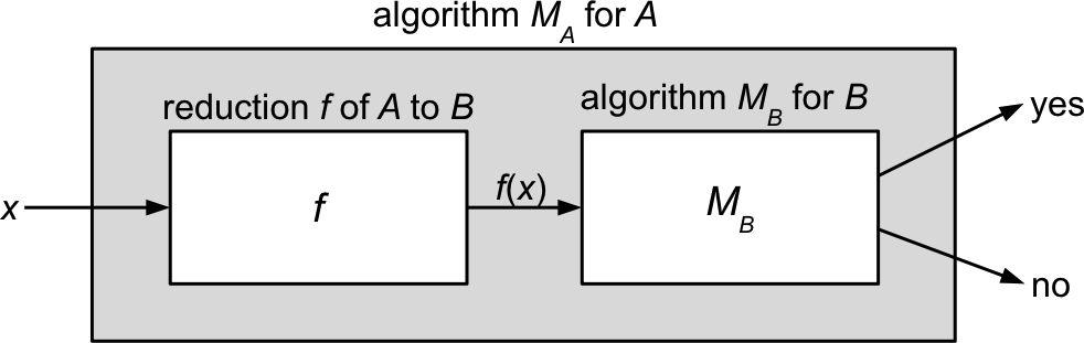
  • Since \(B \in \P\), there is an algorithm \(M_B\) for \(B\) running in time \(O(n^k)\) for some constant \(k\).

  • Since \(A \le^\P B\), there is a reduction \(f\) from \(A\) to \(B\) running in time \(O(n^c)\) for some constant \(c\).

  • We can construct an algorithm \(M_A\) deciding \(A\) simply by composing \(f\) and \(M_B\): \[ M_A(x) = M_B(f(x)) \]
    data/images/complexity/reduction_schematic.png
  • What is the time complexity of \(M_A\)? Let \(n = |x|\).

    • \(O(n^c)\) for \(f(x)\), plus \(O(m^k)\) for \(M_B(f(x))\), where \(m = |f(x)|\).
    • Since \(m = O(|x|^c)\), the full time complexity is: \[ O(n^c) + O(O(|x|^c)^k) \fragment{= O(n^c + n^{ck})} \fragment{= O(n^{ck})} \fragment{\quad \implies \quad A \in \P} \]

Implications of \(A \le^\P B\)

Let’s now formalize what we mean by “\(B\) is at least as hard as \(A\)”

Theorem: If \(A \le^\P B\) and \(B \in \P\), then \(A \in \P\). (“if \(B\) is easy, then \(A\) is easy”)

  • If the fastest algorithm for \(B\) runs in time \(t(n)\), then the fastest algorithm for \(A\) takes no more than \(p(n) + t(p(n))\) where \(p(n)\) is the polynomial running time of \(f\).
  • These runtimes are both “polynomially equivalent.”

Corollary: If \(A \le^\P B\) and \(A \notin \P\), then \(B \notin \P\).

This corollary is the way we typically use reductions:
we know/believe \(A\) is hard, and want to show \(B\) is also hard.

Which direction to reduce

Suppose we want to show that \(\probSAT\) is at least as hard as \(\probHamPath\).

Which problem should we reduce to which?

\[ \probHamPath \le^\P \probSAT \]

\[ \probHamPath \overset{f}{\longrightarrow} \probSAT \]

  • We equivalently want to show \(\probHamPath\) is “at least as easy” as \(\probSAT\).
  • We do this by exhibiting an algorithm for \(\probHamPath\):
    • Reduce to \(\probSAT\) via \(f\).
    • Run the algorithm for \(\probSAT\).

Reductions between problems of different types

  • The reduction from \(\probClique\) to \(\probIndSet\) (and vice versa) was not too surprising since the concepts of cliques and independent sets are closely related.
  • But reductions can remarkably creative, drawing connections between seemingly unrelated problems.
  • To see this, let’s consider another problem known to be as hard as \(\probSAT\), called \(\probThreeSAT\).
  • \(\probThreeSAT\) is a special case of \(\probSAT\) where the Boolean formula is in a special form.

Reductions between problems of different types: \(\probThreeSAT\)

A Boolean formula is in conjunctive normal form (CNF) if it is a conjunction of clauses,
where each clause is a disjunction of literals (“literal” = variable or its negation). Example:

\[ \phi = \underbrace{(x \lor \overline{y} \lor \overline{z} \lor w)}_\text{clause 1} \land \underbrace{(z \lor \overline{w} \lor x)}_\text{clause 2} \land \underbrace{(y \lor \overline{x})}_\text{clause 3} \]

\(\encoding{\phi} \in \probSAT\) iff, for every clause, we can make at least one literal true.

A Boolean CNF formula \(\phi\) is a 3-CNF formula if each of its clauses has exactly 3 literals.
Example: \[ \phi = (x \lor \overline{y} \lor \overline{z}) \land (z \lor \overline{y} \lor x) \]

\[ \probThreeSAT = \setbuild{\encoding{\phi}}{\phi \text{ is a satisfiable 3-CNF formula}} \]

This turns out to be just as hard as \(\probSAT\)!

Reductions between problems of different types: \(\probThreeSAT\)

\[ \probThreeSAT = \setbuild{\encoding{\phi}}{\phi \text{ is a satisfiable 3-CNF formula}} \]

\[ \probIndSet = \setbuild{\encoding{G, k}}{ G \text{ is an undirected graph with a } k\text{-independent set}} \]

  • We’ll now show that \(\probIndSet\) is at least as hard as \(\probThreeSAT\). \[ \probThreeSAT \le^\P \probIndSet \]
  • This is not obvious how to do: \(\probIndSet\) involves graphs and \(\probThreeSAT\) involves formulas.
  • Our reduction will need to convert clauses of a 3-CNF formula into graph structures.
  • These structures built by the reduction are called gadgets
    • The literals of the formula will be “simulated” by nodes in the graph.
    • The clauses will be “simulated” by triplets of nodes.

Reductions between problems of different types: \(\probThreeSAT\)

\[ \probThreeSAT = \setbuild{\encoding{\phi}}{\phi \text{ is a satisfiable 3-CNF formula}} \]

\[ \probIndSet = \setbuild{\encoding{G, k}}{ G \text{ is an undirected graph with a } k\text{-independent set}} \]

Theorem: \(\probThreeSAT \le^\P \probIndSet\).

Proof:

  • Given a 3-CNF formula \(\phi\), our reduction must produce a pair \((G, k)\) such that: \[ \encoding{\phi} \in \probThreeSAT \; \iff \; \encoding{G, k} \in \probIndSet \]

  • Set \(k\) equal to the number of clauses in \(\phi\).

  • Write \(\phi\) as: \[ \phi = (a_1 \lor b_1 \lor c_1) \land (a_2 \lor b_2 \lor c_2) \land \ldots \land (a_k \lor b_k \lor c_k) \] where \(a_i, b_i, c_i\) are the three literals in clause \(i\).

G will have \(3k\) nodes,
one for each literal in \(\phi\).

Example gadget construction

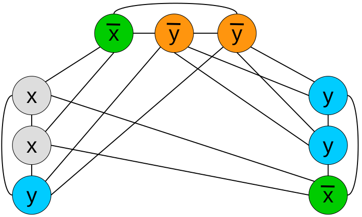
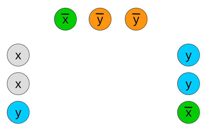
\[ \phi = (x \lor x \lor y) \land (\overline{x} \lor \overline{y} \lor \overline{y}) \land (\overline{x} \lor y \lor y) \hspace{6em} \]

Is this formula satisfiable?
Yes: \(x = 0, y = 1\).

\(\encoding{\phi} \in \probThreeSAT\) iff we can pick
one literal from each clause
to set to “1” without conflicts!
data/images/complexity/3sat-IS-reduction-no-edges.svg data/images/complexity/3sat-IS-reduction-only-triple-edges.svg data/images/complexity/3sat-IS-reduction.svg

Reductions between problems of different types: \(\probThreeSAT\)

Theorem: \(\probThreeSAT \le^\P \probIndSet\).

Proof:

  • Given a 3-CNF formula \(\phi\): \[ \phi = (a_1 \lor b_1 \lor c_1) \land (a_2 \lor b_2 \lor c_2) \land \ldots \land (a_k \lor b_k \lor c_k) \] we produce a pair \((G, k)\) such that: \[ \encoding{\phi} \in \probThreeSAT \; \iff \; \encoding{G, k} \in \probIndSet \]

  • Set \(k\) equal to the number of clauses in \(\phi\).

  • Create one node in \(G\) for each literal in \(\phi\). data/images/complexity/3sat-IS-reduction-no-edges.svg
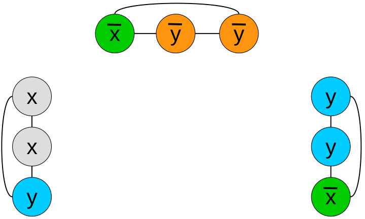
  • Create edge {u, v} in \(G\) if and only if:
    • \(u\) and \(v\) correspond to literals in the same clause (triple), or data/images/complexity/3sat-IS-reduction-only-triple-edges.svg
    • \(u\) is labeled \(x\) and \(v\) is labeled \(\overline{x}\) for some variable \(x\) (or vice versa). data/images/complexity/3sat-IS-reduction.svg

We can generate these edges in polynomial time by looping over all pairs of nodes (\(O(|V|^2)\))
and checking the these two conditions by scanning through \(\phi\). (Python code in lecture notes)

Reductions between problems of different types: \(\probThreeSAT\)

data/images/complexity/3sat-IS-reduction.svg

Proof that \(\encoding{\phi} \in \probThreeSAT \; \iff \; \encoding{G, k} \in \probIndSet\):

  • \(\phi\) satisfiable \(\implies\) \(G\) has a \(k\)-independent set.
    • Suppose \(\phi(w) = 1\) (\(w\) is a satisfying assignment)
    • Then \(w\) makes at least one literal in each clause true.
    • Construct \(k\)-independent set \(S\) by selecting one node from each clause labeled by a true literal. (break ties arbitrarily)
    • For every \(u, v \in S\):
      • in different triples (so not connected by edge type 1)
      • not labeled by variables \(a\) and \(\overline{a}\) respectively (so not connected by edge type 2)
    • So \(u\) and \(v\) are not connected by an edge, so \(S\) is a \(k\)-independent set in \(G\)!
  • \(G\) has a \(k\)-independent set \(\implies\) \(\phi\) satisfiable
    • Given an \(k\)-independent set \(S\), choose assignment \(w\) by setting variable \(a\) to true if some node in \(S\) is labeled \(a\) and false if labeled \(\overline{a}\).
      • If some neither literal \(a\) nor \(\overline{a}\) appears in \(S\), set \(a\) arbitrarily.
    • Every node in \(S\) must correspond to a different clause due to edge type \(1\).
    • Since there are \(k\) clauses and \(|S| = k\), each clause must have at least one true literal marked.
    • The edges in \(G\) between nodes for “conflicting” literals mean \(w\) does not set \(a\) and \(\overline{a}\) to true at the same time for any \(a\), so \(w\) is a satisfying assignment for \(\phi\)!

Recall: Definition of polynomial-time reducibility

Let \(A, B \subseteq \binary^*\) be decision problems. We say \(A\) is polynomial-time reducible to \(B\)
if there is a polynomial-time computable function \(f\) such that for all \(x \in \binary^*\):

\[ x \in A \iff f(x) \in B \]

We denote this by \(A \le^P B\).

\(A \le^P B\) means: “B is at least as hard as A” (to within a polynomial-time factor).

  • If \(A \le^P B\) and \(B \in \P\) then \(A \in \P\).
  • If \(A \le^P B\) and \(A \notin \P\) then \(B \notin \P\).

Reductions don’t themselves solve problems!

data/images/complexity/reduction_schematic.png

  • A reduction \(f\) is just a (polynomial-time) algorithm
  • It enables solving problem \(A\) in terms of an algorithm for problem \(B\).
  • However, \(f\) does not itself solve either problem!
    • It transforms an instance of problem \(A\) (e.g., a formula for \(\probThreeSAT\))
      into an instance of problem \(B\) (e.g., a graph for \(\probIndSet\)).
    • It preserves the “yes” or “no” answer to the original problem
      (but does not provide the answer itself).