Title
Undecidability of the halting problem
So far we have assumed that the halting problem is undecidable: \[ \probHALT = \setbuild{\encoding{M, w}}{M \text{ is a Turing machine that halts on } w} \] and used this to prove that other problems are undecidable using Turing reductions.
- We will prove that the halting problem is undecidable using Turing’s original 1936 proof.
- Turing’s proof was based on the diagonalization technique originally developed by Cantor to prove the existence of different sizes of infinity.
- There are an infinite number of reals in \(\R\) and natural numbers in \(\N\)
- But actually the infinite size of \(\R\) is larger than the infinite size of \(\N\) in a rigorous sense.
- We will warm up to this by studying the sizes of sets.
Recall: 1-1 and onto functions
- A function \(f: D \to R\) is 1-1 (pronounced “one to one”, a.k.a., injective)
if every element in \(D\) maps to a unique element in \(R\).- \(f(a) = f(b) \implies a = b\); equivalently \(a \ne b \implies f(a) \ne f(b)\).
- A function \(f: D \to R\) is onto (a.k.a., surjective)
if every element in \(R\) is the image of some element in \(D\).- For every \(r \in R\), there is \(d \in D\) such that \(f(d) = r\).
- A function that is both one-to-one and onto
is called bijective.
Comparing the sizes of sets
- How can we compare the sizes of two sets?
- For finite sets, we can just count the number of elements in each set and compare.
But this breaks down for infinite sets! - To compare \(\N\) and \(\R\), we might be tempted to claim \(\N\) is obviously smaller since \(\N \subsetneq \R\).
- But checking if \(A \subsetneq B\) is a bad way to determine whether \(|A| < |B|\).
- Clearly \(|\{1, 2\}| < |\{3, 4, 5\}|\), but \(\{1, 2\} \not \subseteq \{3, 4, 5\}\).
- Many sets have a clear size relationship without one being a subset of the other.
- Also, \(\N \subsetneq \Z\), but actually we will see that \(\N\) and \(\Z\) are the “same size.”
- Cantor’s idea was to compare sets by finding correspondences between them.
- Two finite sets \(A\) and \(B\) are the same size if and only if we can find a bijection between them.
- Furthermore, \(|A| < |B|\) if and only if there is no onto function \(f: A \to B\).
(Equivalently, there is no injective function \(f: B \to A\).)
No onto function exists, so
\(|\{1, 2\}| < |\{3, 4, 5\}|\)
Comparing the sizes of sets
We can use this approach of comparing sizes by establishing correspondences to define what it means for one set to be smaller than another:
In the previous example, we can exhibit an onto function from \(\{3, 4, 5\}\) to \(\{1, 2\}\) to conclude \(|\{3, 4, 5\}| \ge |\{1, 2\}|\). \[ f(3) = 1, \quad f(4) = 2, \quad f(5) = 2. \]
But now we can apply the definition to compare infinite sets!
Definition: For any sets \(A\) and \(B\), we write \(|A| \ge |B|\) if and only if there is an onto function \(f: A \to B\).
Onto vs 1-1 functions
Observation: For any sets \(A\) and \(B\), there is an onto function \(f: A \to B\) if and only if there is a 1-1 function \(g: B \to A\).
Proof:
- (\(\implies\)): Let \(f: A \to B\) be onto.
- We construct a 1-1 function \(g: B \to A\) as follows:
- Since \(f\) is onto, for each \(b \in B\), there’s at least one \(a \in A\) such that \(f(a) = b\).
- Define \(g(b)\) to be any such \(a\).
- Since \(f\) is a function, for each \(a \in A\), there is a unique \(b \in B\) such that \(f(a) = b\).
- Therefore, for any \(b_1, b_2 \in B\) with \(b_1 \ne b_2\), we have \(g(b_1) \ne g(b_2)\), so \(g\) is 1-1.
- We construct a 1-1 function \(g: B \to A\) as follows:
- (\(\impliedby\)): Let \(g: B \to A\) be 1-1.
- We construct an onto function \(f: A \to B\) as follows:
- For each \(a \in A\), if there exists \(b \in B\) such that \(g(b) = a\), define \(f(a) = b\) (there is at most one such \(b\) since \(g\) is 1-1).
- Otherwise, define \(f(a)\) to be an arbitrary element \(b_0 \in B\).
- Since \(g\) is 1-1, for each \(b \in B\), there exists at most one \(a \in A\) such that \(g(b) = a\).
- Therefore, for any \(b \in B\), there exists at least one \(a \in A\) such that \(f(a) = b\), so \(f\) is onto.
- We construct an onto function \(f: A \to B\) as follows:
This justifies stating that \(|B| \le |A|\) if and only if there is a 1-1 function \(g: B \to A\).
Bijections vs onto vs 1-1 functions
Note: It is possible to have 1-1 functions \(f: A \to B\) and \(g: B \to A\) but for neither to be onto; e.g. \(f,g: \N \to \N\) defined by \(f(n)=g(n)=n+1\) or \(2n\).
Bijections vs onto vs 1-1 functions
Schröder-Bernstein Theorem: For any two sets \(A\) and \(B\), there is a bijection \(h: A \to B\) if and only if there are 1-1 functions \(f: A\) \(\to\) \(B\) and \(g: B\) \(\to\) \(A\).
Proof:
- (\(\implies\)): Since \(h\) is a bijection, it is 1-1 (let \(f = h\)) and so is its inverse (let \(g = h^{-1}\)).
- (\(\impliedby\)):
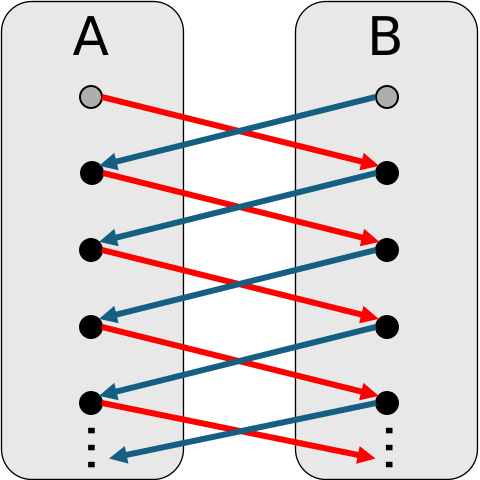
- Define the directed graph \(G=(V,E)\) where \(V=A \cup B\) and \((u,v) \in E\) if either \(f(u) = v\) or \(g(u) = v\).
- Each node has outdegree exactly 1 (\(f\) and \(g\) are functions) and indegree at most 1 (\(f\) and \(g\) are 1-1).
- So \(G\) has four types of connected components:
- Finite cycles: \(\fragment{a_0}\) \(\stackrel{f}{\to}\) \(b_0\) \(\stackrel{g}{\to}\) \(a_1\) \(\stackrel{f}{\to}\) \(b_1\) \(\stackrel{g}{\to}\) \(\dots a_k\) \(\stackrel{f}{\to}\) \(b_k\) \(\stackrel{g}{\to}\) \(a_0\)
- Bi-infinite paths: \(\dots a_{-2}\) \(\to\) \(b_{-2}\) \(\to\) \(a_{-1}\) \(\to\) \(b_{-1}\) \(\to\) \(a_0\) \(\to\) \(b_0\) \(\to\) \(a_1\) \(\to\) \(b_1\) \(\to\) \(a_2\) \(\to\) \(b_2\) \(\to\) \(\dots\)
- One-way infinite paths with left endpoint in \(A\): \(a_0\) \(\to\) \(b_0\) \(\to\) \(a_1\) \(\to\) \(b_1\) \(\to\) \(a_2\) \(\to\) \(b_2\) \(\to\) \(\dots\)
- One-way infinite paths with left endpoint in \(B\): \(a_0\) \(\to\) \(b_0\) \(\to\) \(a_1\) \(\to\) \(b_1\) \(\to\) \(a_2\) \(\to\) \(b_2\) \(\to\) \(\dots\)
- For each type of connected component \(C \subseteq A \cup B\), we’ll define a bijection \(h_C: A \cap C \to B \cap C\), and \(h\) will be the union of all these bijections.
Bijections vs onto vs 1-1 functions
Schröder-Bernstein Theorem: For any two sets \(A\) and \(B\), there is a bijection \(h: A \to B\) if and only if there are 1-1 functions \(f: A\) \(\to\) \(B\) and \(g: B\) \(\to\) \(A\).
Proof: We must define a bijection \(h_C: A \cap C \to B \cap C\) for each connected component \(C\).
- Case 1: \(C\) is a finite cycle \(a_0\) \(\to\) \(b_0\) \(\to\) \(a_1\) \(\to\) \(b_1\) \(\to\) \(\dots a_k\) \(\to\) \(b_k\) \(\to\) \(a_0\).
- Let \(h_C(a_i) = f(a_i) = b_{i}\); \(h_C\) is 1-1 since \(f\) is, and \(h_C\) is onto since every \(b\) in the cycle is \(f(a)\) for some \(a\) in the cycle.
- Case 2: \(C\) is a bi-infinite path \(\dots a_{-2}\) \(\to\) \(b_{-2}\) \(\to\) \(a_{-1}\) \(\to\) \(b_{-1}\) \(\to\) \(a_0\) \(\to\) \(b_0\) \(\to\) \(a_1\) \(\to\) \(b_1\) \(\to\) \(a_2\) \(\to\) \(b_2\) \(\to\) \(\dots\)
- Let \(h_C(a_i) = f(a_i) = b_i\) … same argument as Case 1!
- Case 3: \(C\) is a one-way infinite path with left endpoint in \(A\): \(a_0\) \(\to\) \(b_0\) \(\to\) \(a_1\) \(\to\) \(b_1\) \(\to\) \(a_2\) \(\to\) \(b_2\) \(\to\) \(\dots\)
- Let \(h_C(a_i) = f(a_i) = b_i\) … same argument again!
- Case 4: \(C\) is a one-way infinite path with left endpoint in \(B\): \(a_0\) \(\to\) \(b_0\) \(\to\) \(a_1\) \(\to\) \(b_1\) \(\to\) \(a_2\) \(\to\) \(b_2\) \(\to\) \(\dots\)
- Let \(h_C(a_i) = g^{-1}(a_i) = b_{i}\); note \(g^{-1}\) is well-defined since \(g\) is 1-1.
- Note this is like saying: reverse all the edges in \(C\) to get \(b_0\) \(\leftarrow\) \(a_0\) \(\leftarrow\) \(b_1\) \(\leftarrow\) \(a_1\) \(\leftarrow\) \(b_2\) \(\leftarrow\) \(a_2\) \(\leftarrow\) \(\dots\), and then (like the other cases) just map each node to its out-neighbor; this is the only case where \(h\) is defined by blue edges (\(g\)) instead of red edges (\(f\)).
- \(h_C\) is 1-1 since \(g^{-1}\) is, and \(h_C\) is onto since every \(b\) in the path is \(g^{-1}(a)\) for some \(a\) in the path.
- Let \(h_C(a_i) = g^{-1}(a_i) = b_{i}\); note \(g^{-1}\) is well-defined since \(g\) is 1-1.
The Schröder-Bernstein Theorem, and the previous observation, justifies stating that for any sets \(A,B\),
\(|A| = |B|\) \(\iff\) \(\exists h: A \stackrel{\text{1-1,onto}}{\to} B\) \(\iff\) \(\exists f: A \stackrel{\text{1-1}}{\to} B, g: B \stackrel{\text{1-1}}{\to} A\) \(\iff\) \(\exists f: A \stackrel{\text{onto}}{\to} B, g:B \stackrel{\text{onto}}{\to} A\).
\(|\N|\) vs. \(|\Z|\)
- Recall that \(\N\) denotes the set of nonnegative integers, and \(\Z\) denotes all integers. \[ \N = \{0, 1, 2, \ldots\}, \quad \quad \Z = \{\ldots, -2, -1, 0, 1, 2, \ldots\} \]
- To compare their sizes, we look for onto functions between them.
- It is easy to find onto functions from \(\Z\) to the “obviously smaller” \(\N\). So \(|\Z| \ge |\N|\).
- What’s a good choice for \(f\)? \(f(n) = \abs{n}\)
- Many other choices are possible, e.g. \(f(n) = \max(n, 0)\).
- In fact, whenever \(A \subseteq B\) we can construct an onto function \(f: B \to A\) (i.e., if \(A \subseteq B\) then \(|A| \le |B|\)): \[ f(x) = \begin{cases} x & \text{ if } x \in A \\ a_0 & \text{otherwise.} \end{cases}, \quad \quad \text{where } a_0 \in A \text{ is arbitrary.} \]
- \(f(n) = \max(n, 0)\) is an example of this general construction for \(B = \Z\) and \(A = \N\), with \(a_0 = 0\).
Can we find an onto function from \(\N\) to \(\Z\)? (showing \(|\N| \ge |\Z|\))
\(|\N|\) vs. \(|\Z|\)
- Recall that \(\N\) denotes the set of nonnegative integers, and \(\Z\) denotes all integers. \[ \N = \{0, 1, 2, \ldots\}, \quad \quad \Z = \{\ldots, -2, -1, 0, 1, 2, \ldots\} \]
- To compare their sizes, we look for onto functions between them.
- It is easy to find onto functions from \(\Z\) to the “obviously smaller” \(\N\). So \(|\Z| \ge |\N|\).
We can find an onto function \(f:\N \to \Z\) by letting \(f(0)=0\) and \(f(1), f(2), f(3), f(4), \dots\) alternate positive and negative integers. \[ \fragment{\begin{array}{cccccccccccccc} \\ & & & & & 0 & 1 & 2 & 3 & 4 & \cdots \\ \\ \cdots &\stackrel{f(8)=}{-4} & \stackrel{f(6)=}{-3} & \stackrel{f(4)=}{-2} & \stackrel{f(2)=}{-1} & \stackrel{f(0)=}{0} & \stackrel{f(1)=}{1}& \stackrel{f(3)=}{2}& \stackrel{f(5)=}{3}& \stackrel{f(7)=}{4}& \cdots \end{array}} \]
\[ \fragment{ f(n) = \begin{cases} -\frac{n}{2} & \text{ if } n \text{ is even.} \\ \left \lceil \frac{n}{2} \right \rceil & \text{ if } n \text{ is odd} \end{cases} } \]
Thus also \(|\N| \ge |\Z|\), and so \(|\N| = |\Z|\).
Enumerating sets no bigger than \(\N\)
- Showing an onto function \(f:\N \to A\) means showing \(A = \{f(0), f(1), f(2), \dots\}\)
- Equivalently, there is a one-way infinite sequence \((a_0 = f(0), a_1 = f(1), a_2=f(2), \dots )\) containing every element of \(A\).
- This is called an enumeration of \(A\).
- It’s okay if elements of \(A\) appear multiple times in the sequence.
- This is one reason an older term for “countable” (which we will define to mean \(|A| \le |\N|\)) is “enumerable”.
- Side note: computably enumerable (c.e.), i.e., Turing recognizable, sets can be characterized as sets where this function \(f\) is computable.
\(|\N|\) vs. \(|\Q|\)
Let’s now consider the rational numbers \(\Q\). \[ \Q = \setbuild{\frac{n}{d}}{n \in \Z, d \in \N^+ } \]
It looks like there are way more of these!
We’ll start out with just the positive rationals \(\Q^+\).
Clearly \(|\Q^+| \ge |\N^+|\) since \(\N^+ \subsetneq \Q^+\), and thus \(|\Q^+| \ge |\N|\).
Example function showing \(|\N^+| \ge |\N|\)?
\(|\N|\) vs. \(|\Q|\)
Let’s now consider the rational numbers \(\Q\). \[ \Q = \setbuild{\frac{n}{d}}{n \in \Z, d \in \N^+ } \]
It looks like there are way more of these!
We’ll start out with just the positive rationals \(\Q^+\).
Clearly \(|\Q^+| \ge |\N^+|\) since \(\N^+ \subsetneq \Q^+\), and thus \(|\Q^+| \ge |\N|\).
- But what about finding an onto \(f : \N \to \Q^+\)?
- How can we enumerate \(\Q^+\)?
The following won’t work: \[ \frac{1}{1}, \; \fragment{\frac{1}{2},} \; \fragment{\frac{1}{3},} \; \fragment{\frac{1}{4}, \; \cdots,} \; \fragment{\frac{2}{1}, \; \frac{2}{2}, \; \frac{2}{3}, \; \frac{2}{4}, \; \cdots, \; \frac{3}{1}, \; \frac{3}{2}, \; \frac{3}{3}, \; \frac{3}{4}, \; \cdots} \hspace{20em} \]
Larger numerators aren’t reached at any finite step! Numerator and denominator must change together!
\(|\N|\) vs. \(|\Q|\)
Let’s now consider the rational numbers \(\Q\). \[ \Q = \setbuild{\frac{n}{d}}{n \in \Z, d \in \N^+ } \]
It looks like there are way more of these!
We’ll start out with just the positive rationals \(\Q^+\).
Clearly \(|\Q^+| \ge |\N^+|\) since \(\N^+ \subsetneq \Q^+\), and thus \(|\Q^+| \ge |\N|\).
- But what about finding an onto \(f : \N \to \Q^+\)?
- How can we enumerate \(\Q^+\)?
- We can list them in order of \(n + d\)!
- \(\fragment{\overbrace{\frac{1}{1}}^{n+d=2}, \quad } \; \fragment{\overbrace{\frac{1}{2}, \; \frac{2}{1}}^{n+d=3},} \quad \; \fragment{\overbrace{\frac{3}{1}, \; \frac{2}{2}, \; \frac{1}{3}}^{n+d=4}, \quad} \; \fragment{\overbrace{\frac{4}{1}, \; \frac{3}{2}, \; \frac{2}{3}, \; \frac{1}{4}}^{n+d=5}, \; \quad \cdots}\)
- This way every positive rational is eventually reached.
| 1 | 2 | 3 | 4 | |
|---|---|---|---|---|
| 1 | 1/1 | 2/1 | 3/1 | 4/1 |
| 2 | 1/2 | 2/2 | 3/2 | 4/2 |
| 3 | 1/3 | 2/3 | 3/3 | 4/3 |
| 4 | 1/4 | 2/4 | 3/4 | 4/4 |
\(|\N|\) vs. \(|\Q|\)
- We’ve now shown the existence of an onto function \(f: \N \to \Q^+\).
- Therefore \(|\N| \ge |\Q^+|\) (and thus \(|\N| = |\Q^+|\)).
- What about \(|\Q|\)?
- We can use \(f\) to construct a new onto function \(g: \N \to \Q\). (Similar to trick we used for \(f: \N \stackrel{\text{onto}}{\to} \Z\).) \[ \begin{aligned} g(0) &= 0, \\ g(1) &= \phantom{-}f(0), \\ g(2) &= -f(0), \\ g(3) &= \phantom{-}f(1), \\ g(4) &= -f(1), \\ g(5) &= \phantom{-}f(2), \\ g(6) &= -f(2), \\ \vdots & \\ \end{aligned} \quad \quad \fragment{ g(n) = \begin{cases} 0 & \text{ if } n = 0 \\ f\left(\frac{n+1}{2}\right) & \text{ if } n \text{ is odd} \\ -f\left(\frac{n}{2}\right) & \text{ if } n \text{ is even} \end{cases}} \]
- Since \(f\) maps onto every positive rational, \(g\) maps onto every rational number.
- Hence \(|\N| \ge |\Q|\) (thus \(|\N| = |\Q|\)).
\(|\N|\) vs. \(|\binary^*|\)
- We can also compare sizes of sets don’t just contain numbers!
- For example: let’s compare \(\N\) with the set of all binary strings \(\binary^*\).
- Recall we can do this by enumerating the binary strings.
- We’ve already seen this enumeration! It’s the length-lexicographic ordering: \[ \emptystring, 0, 1, 00, 01, 10, 11, 000, 001, 010, 011, 100, 101, 110, 111, 0000, 0001, \ldots \]
- We conclude that \(|\N| \ge |\binary^*|\).
- The enumeration above actually represents a bijection so in fact \(|\N| = |\binary^*|\).
Did our earlier enumeration of \(\Q\) correspond to a bijection?
\(|\binary^*|\) vs. {all Turing machines}
- Let \(T\) be the set of all Turing machines.
- Each TM can be represented as a binary string, e.g., the bits of the Unicode symbols you type into the TM simulator.
- Thus \(|\binary^*| \ge |T|\), since there is an onto function \(f: \binary^* \to T\) defined by \(g(x) = M\) if \(x\) encodes a TM (and \(M_0\) for some fixed TM otherwise).
- Equivalently, there is a 1-1 function \(g:T \to \binary^*\), defined by \(g(M) =\) binary encoding of \(M\), also showing \(|\binary^*| \ge |T|\).
- Similarly, if \(S\) is any set of “finitely describable” objects (e.g., Python programs, finite graphs, DFAs, Boolean formulas, etc.), then \(|\binary^*| \ge |S|\).
- If you can encode the objects as binary strings, then they are countable (cardinality at most that of \(\N\)).
\(|\R|\) vs. (open) unit interval \((0, 1)\)
- Now let’s consider some huge sets:
- The set of all real numbers \(\R\).
- The open unit interval \((0, 1) \subsetneq \R\).
- Clearly \(|(0, 1)| \le |\R|\) since \((0, 1) \subsetneq \R\).
- Surprisingly, there are the same number of real numbers in \(\R\) and in \((0, 1)\)!
- We first show the easier fact that \(|(0, 1)| \ge |\R^+|\).
- What function can we use? One example: \(g(x) = \frac{1}{x} - 1\)
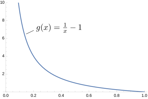
- Note that for any \(y \in \R^+\), we can solve the following for \(x \in (0, 1)\): \[ g(x) = y \quad \iff \quad x = \frac{1}{y + 1}. \]
- What function can we use? One example: \(g(x) = \frac{1}{x} - 1\)
\(|\R|\) vs. (open) unit interval \((0, 1)\)
- Now let’s consider some huge sets:
- The set of all real numbers \(\R\).
- The open unit interval \((0, 1) \subsetneq \R\).
- Clearly \(|(0, 1)| \le |\R|\) since \((0, 1) \subsetneq \R\).
- Surprisingly, there are the same number of real numbers in \(\R\) and in \((0, 1)\)!
- We first show the easier fact that \(|(0, 1)| \ge |\R^+|\).
- Second, we show that \(|\R^+| \ge |\R|\):
- What function can we use? One example: \(f(x) = \log(x)\)
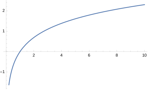
- Note that for any \(y \in \R\), we can solve the following for \(x \in \R^+\): \[ f(x) = y \quad \iff \quad x = e^y. \]
- What function can we use? One example: \(f(x) = \log(x)\)
We conclude that \(|(0, 1)| \ge |\R^+| \ge |\R|\) and so \(|(0, 1)| = |\R|\).
(Open) unit interval \((0, 1)\) vs. \(\{0,1\}^\infty\)
- \(\{0,1\}^\infty\) is the set of all one-way infinite binary sequences.
- “Almost” bijection \(f:\{0,1\}^\infty \to (0,1)\): \(\quad f(S) = 0.S\)
- \(S\) is the binary expansion of a real number in \((0,1)\),
- For example, \(\frac{17}{32} = 2^{-1} + 2^{-4} = 0.\overbrace{1}^{2^{-1}}00\overbrace{1}^{2^{-4}}0000000000000000 \dots\).
- Problem: some reals have two binary expansions
- example above: \(\frac{17}{32} = \begin{array}{cc}0.10010000000000000000\dots&=\\ 0.10001111111111111111\dots&\end{array}\), the so-called dyadic rationals).
- So \(f\) is not 1-1.
- \(f\) is onto, so \(|\{0,1\}^\infty| \ge |(0, 1)|\).
- To see \(|(0, 1)| \ge |\{0,1\}^\infty|\), what’s an onto function \(g:(0,1) \to \{0,1\}^\infty\)?
- For \(x \in (0,1)\), let \(g(x)\) be a binary expansion of \(x\) (choose the one ends in all 0s if it is a dyadic rational).
- Thus \(|\{0,1\}^\infty| = |(0, 1)| \fragment{= |\R|.}\)
\(\{0,1\}^\infty\) vs. \(\mathcal{P}(\N)\)
- Bijection \(h: \{0,1\}^\infty \to \mathcal{P}(\N)\)? (subsets of \(\N\))
- For \(S \in \{0,1\}^\infty\), define \(h(S) = \setbuild{n \in \N}{\text{the } n^\text{th} \text{ bit of } S \text{ is } 1}\).
- \(S\) is known as the characteristic sequence of the set \(h(S) \subseteq \N\).
- For example, \(S = 0 0 \overbrace{1}^2 \overbrace{1}^3 0 \overbrace{1}^5 0 \overbrace{1}^7 0 0 0 \overbrace{1}^{11} 0 \overbrace{1}^{13} 0 0 0 \overbrace{1}^{17} 0 \dots\) is the characteristic sequence of the prime numbers.
- Thus \(|\{0,1\}^\infty| = |\mathcal{P}(\N)|\).
- Recall we showed \(|\N| = |\binary^*|\) earlier, so \(|\{0,1\}^\infty| = |\mathcal{P}(\{0,1\}^*)|\) also.