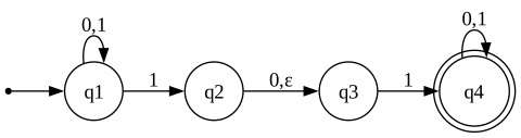
Next model of computation is the Nondeterministic Finite Automaton (NFA).
What’s different here vs. a DFA?
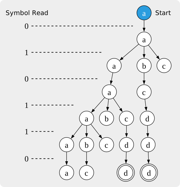
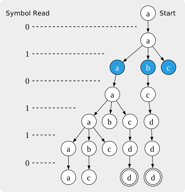
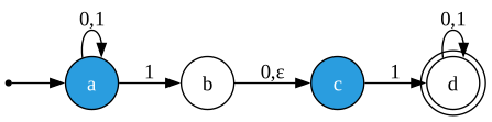
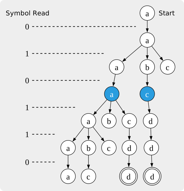
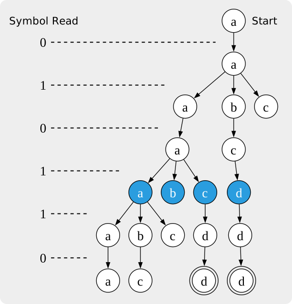
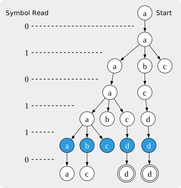
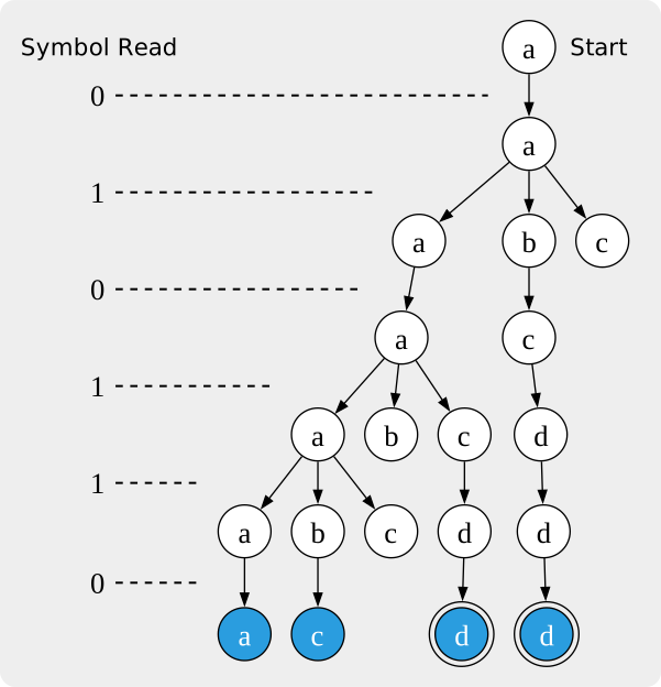
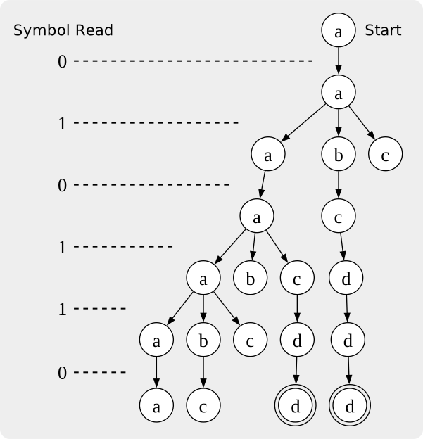
Example processing the string \(010110\):
← Accept!
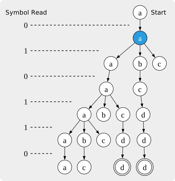
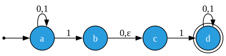
Example processing the string 010110:
010110
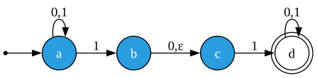
Begin in the state(s) \(\{a\}\).
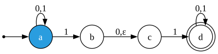
Read 0 and transition to state(s) \(\{a\}\).
010110
Read 1 and transition to state(s) \(\{a, b, c\}\).
010110
Read 0 and transition to state(s) \(\{a, c\}\).
010110
Read 1 and transition to state(s) \(\{a, b, c, d\}\).
010110
Read 1 and transition to state(s) \(\{a, b, c, d\}\).
010110
Read 0 and transition to state(s) \(\{a, c, d\}\).
010110
Since an accept state is highlighted, the NFA accepts the string.
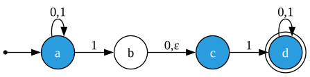
Which of the following strings are accepted by this NFA?
This NFA decides the language: \[\setbuild{w \in \{0, 1\}^*}{w \text{ has 101 or 11 as a substring }}\]
Let’s design an NFA that accepts binary strings with a \(1\) in the third-to-last position: \(\setbuild{w \in \{0, 1\}^*}{w[|w| - 2] = 1}\).
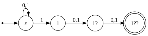
DFA for same language?
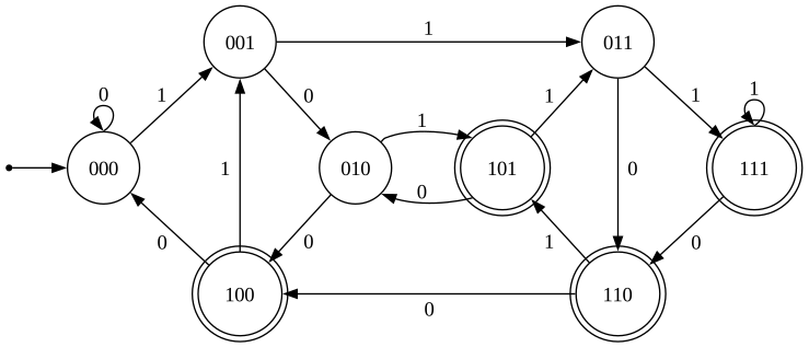
What language over the alphabet \(\{0, 1\}\) does this NFA decide?
Key differences from DFAs that we must encode:
A nondeterministic finite automaton (NFA) is a 5-tuple \((Q, \Sigma, \Delta, s, F)\) where:
For convenience, we can assume that if \(\Delta(q, a)\) is not explicitly defined for \(q \in Q\) and \(a \in \Sigma_\emptystring\), then \(\Delta(q, a) = \emptyset\).
\(Q = \{a, b, c, d\}\)
\(\Sigma = \{0, 1\}\)
\(\Delta\) is defined by the following lookup table:
| \(0\) | \(1\) | \(\emptystring\) | |
|---|---|---|---|
| \(a\) | \(\fragment{\{a\}}\) | \(\fragment{\{a, b\}}\) | \(\fragment{\emptyset}\) |
| \(b\) | \(\fragment{\{c\}}\) | \(\fragment{\emptyset}\) | \(\fragment{\{c\}}\) |
| \(c\) | \(\fragment{\emptyset}\) | \(\fragment{\{d\}}\) | \(\fragment{\emptyset}\) |
| \(d\) | \(\fragment{\{d\}}\) | \(\fragment{\{d\}}\) | \(\fragment{\emptyset}\) |
\(a\) is the start state.
\(F = \{d\}\)
We can equivalently formalize the arrows of the NFA state diagram as a set of transitions.
This is similar to how we defined the productions of a CFG as a set of rules.
This NFA has the transitions:
\[
\{
a \stackrel{0}{\to} a, \quad
a \stackrel{1}{\to} a, \quad
a \stackrel{1}{\to} b, \quad
b \stackrel{0}{\to} c, \quad
b \stackrel{\emptystring}{\to} c,\quad
c \stackrel{1}{\to} d, \quad
d \stackrel{0}{\to} d, \quad
d \stackrel{1}{\to} d
\}
\]
Each of these transitions is formally an ordered triple \((q_i, \sigma, q_j) \in Q \times \Sigma_\emptystring \times Q\) where \(q_i\in Q\) is the source state, \(\sigma \in \Sigma_\emptystring\) is the symbol read, and \(q_j \in Q\) is the destination state.
We can therefore specify the NFA’s transitions as some subset of \(Q \times \Sigma_\emptystring \times Q\).
This formulation makes it easy to talk about adding or removing transitions in the next chapter when we dealing with “constructions”: algorithmic specification of automata.
The finite automaton \(N = (Q, \Sigma, \Delta, q_0, F)\) accepts a string \(w\)
if we can write \(w= y_1 y_2 \ldots y_n \in \Sigma_\emptystring^n\); note possibly \(n>|w|\) since some \(y_i\) may be \(\varepsilon\) and there is a sequence of states \(r_0, r_1, \ldots, r_n \in Q\) such that:
We refer to the sequence \(r_0, r_1, \ldots, r_n\),
or the sequence of transitions followed, as a computation sequence of \(N\) on input \(w\).
\(N\) decides a language \(A\) (denoted \(L(N) = A\)) if \(A = \setbuild{w \in \Sigma^*}{N \text{ accepts } w}\).
A language/decision problem \(A\) is NFA-decidable if there is an NFA \(N\) such that \(L(N) = A\).