Title

ECS 120 Theory of Computation
NP Completeness and Reductions, Pt 3
Julian Panetta
University of California, Davis

Reductions between problems of different types: \(\probThreeSAT\)

\[ \probThreeSAT = \setbuild{\encoding{\phi}}{\phi \text{ is a satisfiable 3-CNF formula}} \]

\[ \probIndSet = \setbuild{\encoding{G, k}}{ G \text{ is an undirected graph with a } k\text{-independent set}} \]

Theorem: \(\probThreeSAT \le^\P \probIndSet\).

Proof:

  • Given a 3-CNF formula \(\phi\), our reduction must produce a pair \((G, k)\) such that: \[ \encoding{\phi} \in \probThreeSAT \; \iff \; \encoding{G, k} \in \probIndSet \]

  • Set \(k\) equal to the number of clauses in \(\phi\).

  • Write \(\phi\) as: \[ \phi = (a_1 \lor b_1 \lor c_1) \land (a_2 \lor b_2 \lor c_2) \land \ldots \land (a_k \lor b_k \lor c_k) \] where \(a_i, b_i, c_i\) are the three literals in clause \(i\).

G will have \(3k\) nodes,
one for each literal in \(\phi\).

Example gadget construction

\[ \phi = (x \lor x \lor y) \land (\overline{x} \lor \overline{y} \lor \overline{y}) \land (\overline{x} \lor y \lor y) \hspace{6em} \]

Is this formula satisfiable?
Yes: \(x = 0, y = 1\).

\(\encoding{\phi} \in \probThreeSAT\) iff we can pick
one literal from each clause
to set to “1” without conflicts!

data/images/complexity/3sat-IS-reduction-no-edges.svg data/images/complexity/3sat-IS-reduction-only-triple-edges.svg data/images/complexity/3sat-IS-reduction.svg

Reductions between problems of different types: \(\probThreeSAT\)

Theorem: \(\probThreeSAT \le^\P \probIndSet\).

Proof:

  • Given a 3-CNF formula \(\phi\): \[ \phi = (a_1 \lor b_1 \lor c_1) \land (a_2 \lor b_2 \lor c_2) \land \ldots \land (a_k \lor b_k \lor c_k) \] we produce a pair \((G, k)\) such that: \[ \encoding{\phi} \in \probThreeSAT \; \iff \; \encoding{G, k} \in \probIndSet \]

  • Set \(k\) equal to the number of clauses in \(\phi\).

  • Create one node in \(G\) for each literal in \(\phi\). data/images/complexity/3sat-IS-reduction-no-edges.svg
  • Create edge {u, v} in \(G\) if and only if:
    • \(u\) and \(v\) correspond to literals in the same clause (triple), or data/images/complexity/3sat-IS-reduction-only-triple-edges.svg
    • \(u\) is labeled \(x\) and \(v\) is labeled \(\overline{x}\) for some variable \(x\) (or vice versa). data/images/complexity/3sat-IS-reduction.svg

We can generate these edges in polynomial time by looping over all pairs of nodes (\(O(|V|^2)\))
and checking the these two conditions by scanning through \(\phi\). (Python code in lecture notes)

Reductions between problems of different types: \(\probThreeSAT\)

data/images/complexity/3sat-IS-reduction.svg

Proof that \(\encoding{\phi} \in \probThreeSAT \; \iff \; \encoding{G, k} \in \probIndSet\):

  • \(\phi\) satisfiable \(\implies\) \(G\) has a \(k\)-independent set.
    • Suppose \(\phi(w) = 1\) (\(w\) is a satisfying assignment)
    • Then \(w\) makes at least one literal in each clause true.
    • Construct \(k\)-independent set \(S\) by selecting one node from each clause labeled by a true literal. (break ties arbitrarily)
    • For every \(u, v \in S\):
      • in different triples (so not connected by edge type 1)
      • not labeled by variables \(a\) and \(\overline{a}\) respectively (so not connected by edge type 2)
    • So \(u\) and \(v\) are not connected by an edge, so \(S\) is a \(k\)-independent set in \(G\)!
  • \(G\) has a \(k\)-independent set \(\implies\) \(\phi\) satisfiable
    • Given an \(k\)-independent set \(S\), choose assignment \(w\) by setting variable \(a\) to true if some node in \(S\) is labeled \(a\) and false if labeled \(\overline{a}\).
      • If some neither literal \(a\) nor \(\overline{a}\) appears in \(S\), set \(a\) arbitrarily.
    • Every node in \(S\) must correspond to a different clause due to edge type \(1\).
    • Since there are \(k\) clauses and \(|S| = k\), each clause must have at least one true literal marked.
    • The edges in \(G\) between nodes for “conflicting” literals mean \(w\) does not set \(a\) and \(\overline{a}\) to true at the same time for any \(a\), so \(w\) is a satisfying assignment for \(\phi\)!

Recall: definition of polynomial-time eeducibility

Let \(A, B \subseteq \binary^*\) be decision problems. We say \(A\) is polynomial-time reducible to \(B\)
if there is a polynomial-time computable function \(f\) such that for all \(x \in \binary^*\):

\[ x \in A \iff f(x) \in B \]

We denote this by \(A \le^P B\).

\(A \le^P B\) means: “B is at least as hard as A” (to within a polynomial-time factor).

  • If \(A \le^P B\) and \(B \in \P\) then \(A \in \P\).
  • If \(A \le^P B\) and \(A \notin \P\) then \(B \notin \P\).

Reductions don’t themselves solve problems!

data/images/complexity/reduction_schematic.png

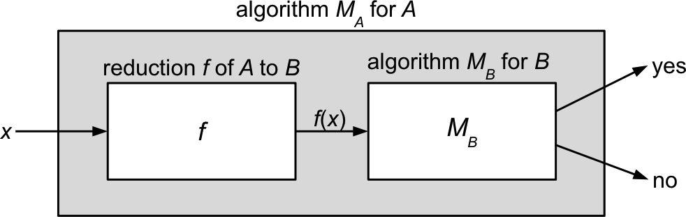
  • A reduction \(f\) is just a (polynomial-time) algorithm
  • It enables solving problem \(A\) in terms of an algorithm for problem \(B\).
  • However, \(f\) does not itself solve either problem!
    • It transforms an instance of problem \(A\) (e.g., a formula for \(\probThreeSAT\))
      into an instance of problem \(B\) (e.g., a graph for \(\probIndSet\)).
    • It preserves the “yes” or “no” answer to the original problem
      (but does not provide the answer itself).

NP-Hardness and NP-Completeness

A language \(B\) is called NP-hard if for every language \(A \in \NP\), \(A \le^P B\).

A language \(B\) is called NP-complete if:

  1. \(B \in \NP\); and
  2. \(B\) is NP-hard.

Theorem: If \(B\) is NP-complete and if \(B \in \P\) then \(\P = \NP\).

Proof:

  • Assume that \(B\) is NP-complete and \(B \in \P\).
  • We know \(\P \subseteq \NP\) and just need to show \(\NP \subseteq \P\).
  • We do this by showing that for any \(A \in \NP\), we have \(A \in \P\).
    • Since \(B\) is NP-hard, we have \(A \le^P B\).
    • Then according to this theorem, \(A \in \P\).

NP-Hardness and NP-Completeness

A language \(B\) is called NP-hard if for every language \(A \in \NP\), \(A \le^P B\).

A language \(B\) is called NP-complete if:

  1. \(B \in \NP\); and
  2. \(B\) is NP-hard.

Theorem: If \(B\) is NP-complete and if \(B \in \P\) then \(\P = \NP\).

Corollary: If \(\P \ne \NP\) then no NP-complete problem is in \(\P\).

This is the significance of NP-completeness:
if you show your problem is NP-hard, then there is (probably) no efficient algorithm for it.

Transitive Property of Polynomial-Time Reducibility

We can chain reductions together!

Observation: \(\le^P\) is transitive
(if \(A \le^P B\) and \(B \le^P C\), then \(A \le^P C\))

def reduce_A_to_B(x):
  """
  reduction from NP prob
  A to NP-hard prob B
  """
  raise NotImplementedError()
def reduce_B_to_C(x):
  """
  reduction from B
  to NP-hard prob C
  """
  raise NotImplementedError()
def C_decider(x):
  """
  hypothetical polynomial-time
  decider
  """
  raise NotImplementedError()
def A_decider(x):
  """
  polynomial time
  """
  y = reduce_A_to_B(x)
  z = reduce_B_to_C(y)
  return C_decider(z)

\(A\) will be a stand-in for any problem in \(\NP\).

Transitive Property of Polynomial-Time Reducibility

Theorem: If \(B\) is \(\NP\)-hard and \(B \le^P C\) for some language \(C\),
then \(C\) is also \(\NP\)-hard.

Proof:

  • Let \(A \in \NP\).
  • Since \(B\) is \(\NP\)-hard, \(A \le^P B\).
  • Since \(\le^P\) is transitive, \(A \le^P C\).
  • Therefore \(C\) is \(\NP\)-hard.

Corollary: If \(B\) is \(\NP\)-complete, \(B \le^P C\),
and \(C \in \NP\), then \(C\) is \(\NP\)-complete.

NP P NP Complete

Finding a reduction from any known-NP-hard problem \(B\) to \(C\) proves that all problems in \(\NP\) are reducible to \(C\)! (\(C\) is NP-hard too.)

Restatement of the Cook-Levin Theorem

Cook-Levin Theorem: \(\probSAT\) and \(\probThreeSAT\) are NP-complete.

  • Proof: Optional Section 10.10 (and ECS 220)
  • This is proved “directly” by exhibiting a reduction from a generic problem \(A \in \NP.\)
  • Once we have these “base” NP-complete problems, we can build up a library of
    NP-complete problems by finding reductions from other problems.

Theorem: \(\probIndSet\) and \(\probClique\) are NP-complete.

Proof:

  • \(\probThreeSAT \le^P \probIndSet\) as proved earlier, so \(\probIndSet\) is NP-hard.
  • \(\probIndSet \le^P \probClique\) as proved earlier, so \(\probClique\) is NP-hard.
  • \(\probClique, \probIndSet \in \NP\) due to polynomial-time verifiers (shown for \(\probClique\) here).
  • Thus, both \(\probIndSet\) and \(\probClique\) are NP-complete.