ECS 120 Theory of Computation

Time complexity and the class P

David Doty (adapted from slides authored by Julian Panetta)

University of California, Davis

Time complexity classes

Can every problem be solved in \(O(n)\), \(O(n^2)\), or maybe \(O(n^{100})\) time
if we simply find the right algorithm?
It turns out, no:
for any time bound \(t\), there are problems that can’t be solved in \(O(t)\),
but can if we allow more time.

“Given more time, a TM can solve more problems!”
We formalize this by introducing notation for “problems solvable in \(O(t)\) time.”

Let \(t: \N \to \N^+\) be a time bound. We define the time complexity class \[ \fragment{\time{t} =} \fragment{\setbuild{L \subseteq \binary^*}{\fragment{L \text{ is decided by a TM with running time } O(t)}}} \]

\(\time{t} \subseteq \powerset(\binary^*)\)

Let \(\REG\) denote the class of regular languages.
True or false: \(\REG \subseteq \time{n}\)

True
False

Time complexity classes

Can every problem be solved in \(O(n)\), \(O(n^2)\), or maybe \(O(n^{100})\) time
if we simply find the right algorithm?
It turns out, no:
for any time bound \(t\), there are problems that can’t be solved in \(O(t)\),
but can if we allow more time.

“Given more time, a TM can solve more problems!”
We formalize this by introducing notation for “problems solvable in \(O(t)\) time.”

Let \(t: \N \to \N^+\) be a time bound. We define the time complexity class \[ \time{t} = \setbuild{L \subseteq \binary^*}{L \text{ is decided by a TM with running time } O(t)} \]

\(\time{t} \subseteq \powerset(\binary^*)\)

For all time bounds \(t_1\) and \(t_2\) such that \(t_1 = O(t_2)\),
\(\time{t_1} \subseteq \time{t_2}\)

True
False

Time complexity classes

Let \(t: \N \to \N^+\) be a time bound. We define the time complexity class \[ \time{t} = \setbuild{L \subseteq \binary^*}{L \text{ is decided by a TM with running time } O(t)} \]

Time Hierarchy Theorem:
Let \(t_1(n)\) and \(t_2(n)\) be time bounds such that \(t_1(n) \log(n) = o(t_2(n))\).
Then \(\time{t_1} \subsetneq \time{t_2}\).

There is a problem that can be solved in \(O(t_2(n))\) time, but not \(O(t_1(n))\) time!

Consequences:

\(\time{n^c} \subsetneq \time{n^{k}}\) for all \(c < k\), e.g., there are problems solvable in quadratic time, but not linear time.
\(\time{n^c} \subsetneq \time{2^{n^\delta}}\) for all \(c, \delta > 0\)
\(\time{2^{cn}} \subsetneq \time{2^{k n}}\) for all \(c < k\)
There is an infinite hierarchy of time complexity classes!

The complexity class \(\P\)

A special time complexity class containing problems with “efficient” solutions:

We denote by \(\P\) the class of languages decidable in polynomial time by a (deterministic) Turing machine: \[ \P = \bigcup_{k = 1}^\infty \time{n^k} \]

Why this notion of efficiency?
- It is robust to changes in our model of computation.
  (All “reasonable” models of computation are polynomially equivalent.)
- Exponential time algorithms are often “brute-force” approaches, while polynomial-time algorithms
  (when they exist) involve deeper insights into the problem. (E.g., Dynamic programming)
- \(\P\) roughly captures the class of problems that are realistically solvable in practice.

Robustness of the definition of \(\P\)

Remember our model of compute time:

The time complexity of a decider \(M\) is the time bound function \(t : \mathbb{N} \to \mathbb{N}^+\) defined as \[ t(n) = \max_{x \in \binary^n} \texttt{time}_M(x), \]

where \(\texttt{time}_M(x)\) is the number of configurations that \(M\) visits on input \(x\).

Specific choices made in this definition:
- \(M\) is a single-tape, deterministic Turing machine.
- \(n\) is the length of the input’s encoding as a binary string.
What if we make different choices?
- If we use a two-tape Turing machine, we would gain at most a quadratic speedup.
  Optional Section 9.3: any \(O(t)\) two-tape TM can be simulated by an \(O(t^2)\) single-tape TM.
  Therefore membership in \(\P\) is unchanged (\(O(n^k) \to O(n^{2k})\))
- Any “reasonable” input encoding also does not change the class \(\P\).

Invariance to “reasonable” input encodings

Let \(\encoding{\mathcal{X}}_1\) and \(\encoding{\mathcal{X}}_2\) be two different encodings of input object \(\mathcal{X}\) into binary strings.
Define an “encoding blowup factor” from \(\encoding{\mathcal{X}}_1\) to \(\encoding{\mathcal{X}}_2\) as: \[ f_{1 \to 2}(n) = \max_{\mathcal{X} \text{ s.t. } |\encoding{\mathcal{X}}_1| = n} |\encoding{\mathcal{X}}_2| \]
If \(f_{1 \to 2}(n) = O(n^c)\) and \(f_{2 \to 1}(n) = O(n^c)\) (i.e., each encoding length is within a polynomial of the other), each encoding yields the same definition of \(\P\).
(Assuming encoding/decoding takes polynomial time.)
Example of reasonable encodings for graph \(G = (V, E)\):
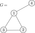
- Node and edge lists:
  \(\encoding{G}_1 = \texttt{ascii\_to\_binary}(((1,2,3,4), ((1,2),(2,3),(3,1),(1,4))))\)
- Binary adjacency matrix: \[ \begin{bmatrix} 0 & 1 & 1 & 1 \\ 1 & 0 & 1 & 0 \\ 1 & 1 & 0 & 0 \\ 1 & 0 & 0 & 0 \\ \end{bmatrix} \quad \Longrightarrow \quad \encoding{G}_2 = 0111101011001000 \hspace{15em} \]

Invariance to “reasonable” input encodings

Let \(\encoding{\mathcal{X}}_1\) and \(\encoding{\mathcal{X}}_2\) be two different encodings of input object \(\mathcal{X}\) into binary strings.
Define an “encoding blowup factor” from \(\encoding{\mathcal{X}}_1\) to \(\encoding{\mathcal{X}}_2\) as: \[ f_{1 \to 2}(n) = \max_{\mathcal{X} \text{ s.t. } |\encoding{\mathcal{X}}_1| = n} |\encoding{\mathcal{X}}_2| \]
If \(f_{1 \to 2}(n) = O(n^c)\) and \(f_{2 \to 1}(n) = O(n^c)\) (i.e., each encoding length is within a polynomial of the other), each encoding yields the same definition of \(\P\).
(Assuming encoding/decoding takes polynomial time.)
Reasonable and unreasonable encodings of \(n \in \N^+\):

\[ \begin{aligned} \encoding{n}_1 \phantom{|} &= \texttt{bin}(n) \in \{0, 1\}^* \\ |\encoding{n}_1| &= \fragment{\lfloor \log_2(n) \rfloor + 1} \fragment{= O(\log n)} \\ \encoding{n}_2 \phantom{|} &= 1^n \\ |\encoding{n}_2| &= n \end{aligned} \hspace{15em} \]

\(f_{1 \to 2}(n) = \fragment{O(2^n)}\)
Dangers of unreasonably inefficient encodings:
- Using exponential time to do simple arithmetic!
- Considering truly exponential-time algorithms to take polynomial time with respect to the input size.

Reasonable encodings of a list of strings \((010, 1001, 11)\)
- ASCII with comma delimiters: 8 * (9 + 2) = 88 bits
- More efficient “bit-doubling” encoding (01 is delimiter): 00 11 00 01 11 00 00 11 01 11 11 (22 bits)

Definition of input size

Formally, the “\(n\)” in time bound \(t(n)\) is the length of the binary encoding \(x = \encoding{\mathcal{X}}\)
We generally want to think of time complexity at a higher level
- For a graph algorithm for \(G=(V,E)\): the complexity in terms of the number of nodes \(n=|V|\); and possibly also edges \(m=|E|\); e.g., Kruskal’s minimum spanning tree algorithm takes time \(O(m \log n)\).
  - But note that an algorithm runs in time polynomial in \(n\) iff it runs in time polynomial in \(n+m\) iff in runs in time polynomial in \(|\encoding{G}|\).
- For a list-processing algorithm: the complexity in terms of the number of elements.
The previous slide shows this distinction doesn’t change membership in \(\P\) provided that \(|\encoding{\mathcal{X}}|\) is a polynomial function of the “intuitive input size.”
Sometimes we still must be careful…
(e.g., when factoring an \(n\)-bit integer, the number of bits is the size!)

Practicality of problems in \(\P\)

The robustness of \(\P\) comes from ignoring the exponents of polynomials.
In practice, this exponent can matter quite a lot!
- In algorithms or scientific computing we care very much about \(O(n^2)\) vs. \(O(n^3)\)
- Even \(O(n^4)\) may be considered too slow for a given application.
However:
- Once we have a polynomial time algorithm, even \(n^{100}\) (“galactic” algorithms), usually someone finds a faster one.
  - Example: first polynomial-time algorithm for deciding if an integer is prime was \(O(n^{12})\), but this was quickly improved to \(O(n^6)\).
- Over time, problems in \(\P\) become much easier to solve due to Moore’s law.
  - Suppose we have an algorithm with time bound \(t(n) = a n^{k}\).
  - Assume we can afford to solve an input of size \(n_0\) in year 0,
    and the number of operations we can afford to run grows by multiplier \(m\) each year.
  - In year \(y\), we can afford to solve inputs of size \(n_0 m^{y / k}\). This is growing exponentially!
  - The size of inputs we can process with exponential time algorithms only grows linearly over time.

Identifying time complexity classes within \(\P\) graphically

If we were to care about the different time complexity classes \(O(n^k)\) within \(\P\)
- How can we visualize their differences?
- How can we experimentally verify that our code has the expected time complexity?
We can try plotting the runtime of our algorithm against different input sizes.
Example: 3sum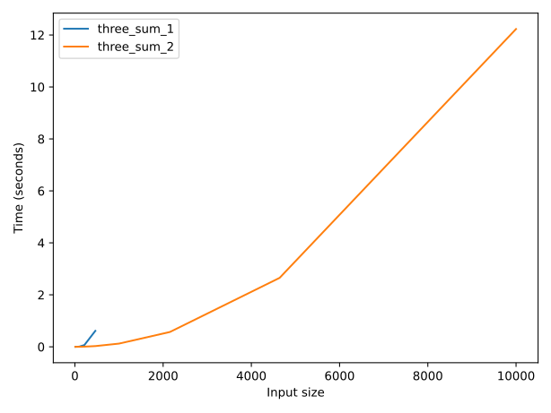

Identifying time complexity classes within \(\P\) graphically

If we were to care about the different time complexity classes \(O(n^k)\) within \(\P\)
- How can we visualize their differences?
- How can we experimentally verify that our code has the expected time complexity?
We can try plotting the runtime of our algorithm against different input sizes.
More specifically, we can use a log-log plot:
Example: 3sum: Slope \(k\) on a log-log plot indicates time complexity \(O(n^k)\).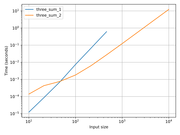

Recall: Time complexity class \(\P\)

We denote by \(\P\) the class of languages decidable in polynomial time by a (deterministic) Turing machine: \(\P = \bigcup_{k = 1}^\infty \time{n^k}\)

Example problem in \(\P\):

3Sum Problem:
Given a set \(A\) of \(n\) integers (\(A \subset \Z\), \(|A| = n\)), check if there are three elements that sum to zero (i.e., \(a + b + c = 0\) for \(a, b, c \in A\)).

  def three_sum_1(A: list[int]) -> bool:
      for i in range(len(A)):
          for j in range(i, len(A)):
              for k in range(j, len(A)):
                  if A[i] + A[j] + A[k] == 0:
                      return True
      return False

Counting the “steps” (innermost line) run: \[ \small \begin{aligned} \text{Total steps} &= \fragment{\sum_{i = 1}^{n} \sum_{j = i}^{n} \sum_{k = j}^{n} 1} \fragment{= \cdots} \fragment{= \frac{n (n + 1) (n + 2)}{6}} \fragment{= O(n^3)} \end{aligned} \]
This is polynomial in the “size” of the input \(n\), so \(3\text{Sum} \in \P\).
Assumes arithmetic operations on integers take \(O(1)\) time.
- Reasonable if integers fit into CPU registers.
- Still true with larger integers, but need more careful argument about efficiency of arithmetic algorithms.

\(\probRelprime\) and the Euclidean algorithm

Integers \(a, b \in \N^+\) are called relatively prime if their greatest common divisor \(\gcd(a, b) = 1\).

\[ \probRelprime = \setbuild{\encoding{a, b}}{ a,b \in \N^+ \text{ and } \gcd(a, b) = 1 } \]

Theorem: \(\probRelprime \in \P\)

Proof: We can compute \(\gcd(a, b)\) efficiently using the Euclidean algorithm: (c. 300 BC!)

def gcd(a: int, b: int) -> int:
    # Order so a ≥ b (simplifies analysis)
    if (a < b): a, b = b, a
    while b > 0:
        a = a % b
        a, b = b, a
    return a

def rel_prime(a: int, b: int) -> bool:
    return gcd(a, b) == 1

Based on the identity: \(\gcd(a, b) = \gcd(a \mod b, b)\).
How many “steps” does this algorithm take?
Count loop iterations (each does constant work).
Each iteration halves the value of the larger number (\(a\))
- Suppose \(b \le \frac{a}{2}\). Then \(a \mod b < b \le \frac{a}{2}\).
- Alternatively, if \(b > \frac{a}{2}\), then \(a \mod b = a - b < \frac{a}{2}\).
So the number of iterations run is at most: \(2 \log_2 a \leq |\encoding{a, b}|\)
This is linear in the size of the input (the number of bits needed to represent \(a\) and \(b\)),
so \(\probRelprime \in \P\).

Simply checking each integer up to \(b\) would take exponential time!

\(\probPath\)

Directed reachability problem:

\[ \probPath = \setbuild{\encoding{G, s, t}}{ G \text{ is a directed graph containing a path from node } s \text{ to } t } \]

Theorem: \(\probPath \in \P \hspace{1em}\) (Use a breadth-first search)

from typing import TypeVar
Node = TypeVar('Node')
type Graph[Node] = tuple[list[Node], list[tuple[Node, Node]]]
def path(G: Graph[Node], s: Node, t: Node) -> bool:
    if s == t: 
        return True
    V, E = G
    seen = {s}
    queue = collections.deque([s])
    while len(queue) > 0:
        node = queue.popleft()
        neighbors = [v for (u,v) in E if u==node]
        for v in neighbors:
            if v == t:
                return True
            if v not in seen:
                seen.add(v)
                queue.append(v)
    return False

What is the asymptotic complexity of this algorithm in terms of \(n = |V|\) and \(m = |E|\)?
How many iterations does the while loop run? At most \(n\) (each node enters queue at most once).
How long does building neighbors take (each itertion)? \(m\) steps (each edge is checked once).
How many total iterations does the for loop run?
At most \(m\): executes once for each edge (since edges populating neighbors list are disjoint between different while loop iterations).

This is \(O(n \cdot m + m)\).
Could we do better?

\(\probConnected\)

Given an undirected graph \(G\), check if it is connected.

\[\probConnected = \setbuild{\encoding{G}}{ G \text{ is connected} }\]

Theorem: \(\probConnected \in \P\)

Simple approach for handling undirected graphs:
convert them to an equivalent directed graph (of proportional size) in polynomial time.

Node = TypeVar('Node')
type Graph[Node] = tuple[list[Node], list[tuple[Node, Node]]]
def add_reverse_edges(G: Graph[Node]) -> Graph[Node]:
    V,E = G
    reverse_edges = [(v,u) for (u,v) in E if (v,u) not in E and (v,u) not in reverse_edges]
    return (V, E+reverse_edges)

Now just check if all pairs of nodes are connected by a path:

def connected(G: Graph[Node]) -> bool:
    V,E = add_reverse_edges(G)
    for (s,t) in itertools.combinations(V,2):
        if not path(G,s,t):
            return False
    return True

\(O(m)\) to build directed version of graph.
\(\binom{n}{2} = \frac{n(n-1)}{2} = O(n^2)\) iterations of forloop.
path takes polynomial time per iteration (previous slides)

\(\probEulerianCycle \in \P\)

Given undirected graph \(G\): does it have an Eulerian cycle? (visiting each edge exactly once)

\[\probEulerianCycle = \setbuild{\encoding{G}}{ G \text{ is an undirected graph with an Eulerian cycle} }\]

Theorem: \(\probEulerianCycle \in \P\)

Proof:

Euler: an undirected graph \(G\) has an Eulerian cycle if and only if every node has an even degree, and all edges belong to a single connected component.

from typing import TypeVar
Node = TypeVar('Node')
type Graph[Node] = tuple[list[Node], list[tuple[Node, Node]]]

def eulerian_cycle(G: Graph[Node]) -> bool:
    V, E = G
    V_pos = [] # nodes with positive degree
    for u in V:
        deg = degree(u, E)
        if deg % 2 == 1: return False
        if deg > 0: V_pos.append(u)
    G_pos = (V_pos, E)
    return connected(G_pos)

def degree(node: Node, E: list[tuple[Node, Node]]) -> int:
    return sum(1 for (u, v) in E if u==node)

degree takes time \(O(m)\).
for loop executes \(n\) iterations, calling degree once each time (other two lines are \(O(1)\)): \(O(nm)\) total.
connected takes polynomial time (previous slides).

Title

Time complexity classes

Time complexity classes

Time complexity classes

The complexity class \(\P\)

Robustness of the definition of \(\P\)

Invariance to “reasonable” input encodings

Invariance to “reasonable” input encodings

Definition of input size

Practicality of problems in \(\P\)

Identifying time complexity classes within \(\P\) graphically

Identifying time complexity classes within \(\P\) graphically

Recall: Time complexity class \(\P\)

Other problems in \(\P\)

\(\probRelprime\) and the Euclidean algorithm

\(\probPath\)

\(\probConnected\)

\(\probEulerianCycle \in \P\)