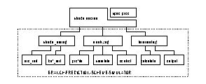
Figure 1. Shade-Based Branch Prediction Scheme Simulator
Branch prediction schemes can be classified into static schemes and dynamic schemes by the way the prediction is made. Static prediction schemes can be simple. The most straight forward one is predicting branches to be always taken by observing that majority of branches are taken. As reported by Lee ad Smith [LS92], this simple strategy can predict correctly 68% of the time. In our study, out of the dynamic instructions traced, 65% of the conditional branches are taken. Our traces also indicate that this simple approach may result in less than 50% correct prediction for some integer programs. Static schemes can also be based on branches' opcodes. Another simple method is using the direction of the branches to make a prediction. If the branch is backward, i.e., the target address is smaller than the PC of the branch instruction, it is predicted to be taken. Otherwise, if the branch is forward, it is predicted to be not taken. This strategy tries to take advantage of loops in the program. It works well for programs with many looping structures. However, it does not work well in the case there are many irregular branches. Profiling is another static strategy which uses previous runs of a program to collect information on the tendencies of a given branch to be taken or not taken and preset a static prediction bit in the opcode of the given branch. Later runs of the program can use this information to make predictions. This strategy suffers from the fact that runs of a program with different input data sets usually result in different branch behaviors. Recently, C. Young and M. Smith proposed static correlated branch prediction(SCBP) trading off increased code size with increased prediction accuracy. At this time, we do not know whether this approach will yield any performance improvement. For more information, refer to [YS94]. In this project, we studied the limit of static approach without code expansion. Our results indicate that the static schemes without code expansion are not comparable to dynamic approaches.
Dynamic schemes are different from static ones in the sense that they use the run-time behavior of branches to make predictions. J. Smith [S81] gave a survey of early simple static and dynamic schemes. The best scheme in his paper is the one which uses 2-bit saturating up-down counters to collect history information which is then used to make predictions. This is perhaps the most well-known technique. McFarling [M93] referred to it as the bimodal branch prediction. There are several variations in the design of the 2-bit counter. Yeh and Patt [YP91] discussed these variations. In many programs with intensive control flow, very often the direction of a branch is affected by the behavior of other branches. By observing this fact, Pan, So, & Rahmeh [PSR92] and Yeh & Patt [YP91] independently proposed correlated branch prediction schemes or two-level adaptive branch prediction schemes. This new approach improved the prediction accuracy by a large factor. Yeh and Patt [YP93] classified the variations of dynamic schemes that using two levels of branch history. McFarling [M93] exploited the possibility of combining branch predictors to achieve even higher prediction accuracy.
Computer technology is advancing at a rapid speed. Advanced VLSI technology makes it possible to have larger branch prediction table and more complicated schemes. The advancement in programming languages also makes it possible to have larger and more complicated programs, and allows more cross-references between branches because of more complicated procedure calls. Multiprocessing and threading become important because of the rise of Multiple Instruction streams, Multiple data streams(MIMD) machines. Therefore, it is important to look at the effect of these advancements on branch prediction.
In this project, we look at some of the following issues. In the literature, there are many MIPS, Alpha, HP-PA, and Power architecture based branch prediction research. We are interested in knowing the impact of a different architecture, SPARC architecture, on branch prediction. Our results do not show any significant, if at all any, impact of architecture on branch prediction. We get similar results as compared to results from previous research. Taking advantage of the fast simulation speed of Shade, we are able to trace much larger programs, try out many different schemes, and experiment with different parameters of the schemes in a reasonable amount of time. We notice that the number of instructions traced clearly affects the resulted branch behavior and prediction accuracy, and that the selection and the size of the testing program set also affects the comparison over different schemes. Since in different applications and programming languages conditional branches behave differently, it is important to have a set of benchmark programs that can truthfully represents the average workload and complexity of the programs people run. We use a partially new collection of programs, which includes 8 SPECint95 beta benchmarks and 13 SPECfp92 benchmarks, to see how well the well-known schemes work on these new programs. We do observe that one new SPEC95 program go has much different branch behavior from previous SPEC programs. In this paper, we first show the performance of several well-known dynamic branch prediction schemes. From the results, we conclude that selective predictor achieves the highest prediction accuracy with the same size of branch prediction buffer. We also observe that conventional static predictors cannot compete with dynamic predictors, and context switching has little impact on branch prediction with today's fast CPU. In addition, complex schemes require longer time to warm up than simple schemes do.
The rest of the report is organized as follows: the related work section gives references to previous work on branch prediction. The design methodology section discusses the methodology used in this study: how the simulated prediction models and testing programs are selected, and how the simulated prediction schemes are designed and implemented. The result analysis section discusses our findings from traces of the benchmark programs. The future work section presents some of the work that may be interesting to explore. The last section summaries the report.
1. Experimental System
Our experiment is conducted on SPARC system 10 with two SuperSparc/60 V8 micro-processors. We compiled c benchmark programs using SUNSoft "cc" version 3.0.1, and compiled fortran programs using SUNSoft "f77" version 3.0.1.
Our data is obtained using "Shade"[SHADE] version 5.15 analyzing programs. Shade is a dynamic code tracer. It links instruction set simulation, trace generation with custom trace analysis. The first advantage of a shade-based simulator over other static trace-based simulators such as pixie based approach is its fast running speed. Shade tends to run fast mainly because the executable being traced, the shade trace generator, and the shade analyzer are all in one single process. The second advantage is that it combines trace generation and trace based analyzer/simulator, thereby avoiding awkward trace file manipulations.
The following figure illustrates the code structure of our shade-based branch prediction simulators.

Figure 1. Shade-Based Branch Prediction Scheme Simulator
2. Benchmark Programs
In different applications and programming languages, conditional branches behave differently. It is important to have a set of benchmark programs that can give a good approximation of the average workload and complexity of the programs that users run. Previous work in this area has been done by tracing the execution of some benchmark programs. In this project, we also use instruction tracing data to measure the performance of different branch prediction schemes. Eight benchmark programs from the beta version of SPEC95 integer program suite and thirteen benchmarks from the SPEC92 floating point program suite are used in this study. Table 1 and 2 list the benchmark programs, their abbreviations that we use, and the testing input data sets used in our experiment.
| SPEC95 Integer Program Beta | ||||
|---|---|---|---|---|
| Benchmark / Input | Dynamic Inst. | Dynamic Cond. Branch | Program / Input size | Static Cond. Branch |
| gcc / 1amptjp.i | 1297M | 221M | 1697K / 222K | 19598 |
| gcc / 1c-decl-s.i | 1297M | 221M | 1697K / 222K | 19603 |
| gcc / 1dbxout.i | 1664M | 28M | 1697K / 42K | 15455 |
| gcc / 1reload1.i | 992M | 173M | 1697K / 148K | 19673 |
| gcc / cccp.i | 1298M | 223M | 1697K / 162K | 19514 |
| gcc / insn-emit.i | 147M | 23M | 1697K / 48K | 10815 |
| gcc / stmt-protoize.i | 986M | 165M | 1697K / 185K | 19746 |
| ghost / convolution.ps-color | 1400M | 238M | 584K / 218K | 4262 |
| ghost / convolution.ps-mono | 1342M | 229M | 584K / 218K | 4312 |
| ghost / convolution.ps-tiff | 1315M | 222M | 584K / 218K | 4330 |
| go / restart.in* | 4535M | 500M | 390K / | 5761 |
| go / neardone.in | 733M | 78M | 390K / | 4874 |
| go / null.in* | 4531M | 500M | 390K / | 5742 |
| m88ksim / dcrand.in* | 7007M | 1000M | 389K / 66K | 824 |
| numi / numi.in* | 7507M | 1000M | 31K / | 1064 |
| li/li-input.lsp* | 12355M | 1000M | 299K / | 1412 |
| perl / jumble.perl* | 3471M | 500M | 400K / | 2523 |
| perl / primes.perl* | 4762M | 500M | 400K / | 2218 |
| vortex / vortex.in* | 7195M | 1000M | 867K / | 7602 |
Table 1. SPEC95 Integer Program Beta and Input Data Description.
| SPEC92 Floating Point Program | ||||
|---|---|---|---|---|
| Benchmark | Dynamic Inst. | Dynamic Cond. Branch | Program size | Static Cond. Branch |
| alvinn | 6792M | 480M | 9612 | 1032 |
| doduc | 1644M | 87M | 247K | 2330 |
| ear | 14506M | 705M | 59K | 1238 |
| fpppp | 8463M | 106M | 138K | 1332 |
| hydro2d | 6627M | 680M | 111K | 2356 |
| mdljdp2 | 4206M | 309M | 79K | 1458 |
| mdljsp2 | 3011M | 338M | 98K | 1520 |
| nasa7 | 11104M | 217M | 91K | 1889 |
| ora | 2029M | 158M | 24K | 1153 |
| su2cor | 8055M | 165M | 150K | 1863 |
| swm256 | 9862M | 66M | 62K | 1335 |
| tomcatv | 1261M | 31M | 21K | 1036 |
| wave5 | 4331M | 286M | 401K | 1956 |
Table 2. SPEC92 Floating Point Program Description.
3. Branch Prediction Scheme Design
Branch prediction schemes using small buffers of branch history take advantage of the repetitive branch taken/untaken execution behavior, thereby achieving better prediction accuracy than the simple static prediction schemes. For each conditional branch, an appropriate counter is incremented or decremented. The most significant bit of the counter determines the prediction decision. J. Smith [S81] observed that a 2-bit counter empirically provides an appropriate amount of damping to changes in branch direction. A 1-bit counter simply records the last executed branches direction. In addition, 3-bit or higher counters do not appear to offer large cost/benefit advantages over 2-bit counters. We will further discuss the design of 2-bit counter in a later subsection on predictor tuning.
Bimodal branch prediction is the simplest 2-bit counter based dynamic prediction scheme. The branch history table is indexed by the low order address bits in the program counter. The following table illustrates the design of the bimodal prediction scheme.
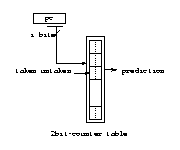
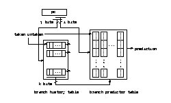 Figure 2, 3. Bimodal Predictor |
Correlation Based Predictor
Correlated branch prediction schemes include common-correlation, gselect, global and local. Since the bimodal scheme takes advantage of the bimodal distribution of branch behavior, it does not perform well when branches have strong dynamic behavior. Correlated prediction schemes are designed to take advantage of relationship between different branch instructions -- certain repetitive branch pattern of several consecutive branches. One correlation based predictor uses two branch history tables. The first table records the history of recent branches -- global history. Each entry is implemented using a shift register. The second table records the branch history for each branch. It is organized as a matrix with rows and columns. Each entry is a 2-bit counter. The pc determines which shift register in the first table and which row of the 2-bit counters of the second table should be used. The chosen global shift register indexes the appropriate counter from the selected row of counters. Prediction is made based the selected counter. The selected shift register and the 2-bit counter will be updated afterwards accordingly. Figure 3 above illustrates the design of correlated schemes.
There are many ways of using pc to index the first and the second tables. Yeh and Patt [YP93] classified these methods into per_address which uses the low order bits of pc and per_set which uses high or middle range bits of pc. They claimed that per_address method and per_set method have similar performance, and the latter has higher implementation cost. We use per_address in our study.
The well-known common-correlation scheme is a correlated scheme that uses a single 2-bit shift register as the global branch history table, and four 2-bit counter for each row of the second table. The 2-bit shift register approach only exploits the correlation between two consecutive branches. Another similar correlated scheme design uses j > 2 bits for the global branch history register and 2^j 2-bit counters for each row of the second table. We adopt the name used by McFarling and refer to it as the gselect scheme. If i equals to 1, i.e. there is just single row in the second table, the scheme is also referred to as the global scheme. Global scheme applies all its buffer for recording the correlation information while ignoring the different branch behavior of a single branch. In most cases, it does not perform as well as other correlated schemes.
More complicated design uses multiple shift registers in the first table. Each register records the branch history of different branches. McFarling referred to it as the local scheme.
Sharing index scheme is referred to as gshare. It was proposed by McFarling. This scheme is similar to the bimodal scheme. It xors a j bits global history shift register with the i bits of the pc before indexing the counter table. Figure 4 illustrates the design of the gshare scheme.
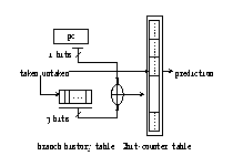
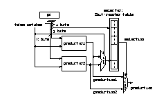 Figure 4, 5. Index Sharing Predictor | Selective Predictor
Different dynamic schemes use different branch history information. Many schemes work well on one type of programs and do not work well on another type of programs. The selective scheme uses two different predictors. Each of two predictors makes prediction independently. A third table is used to track the performance of the two subpredictors and arbitrates which prediction should be used as the final prediction. Selective scheme can perform well on different types of programs. Figure 5 illustrates the design of the selective prediction scheme.
The implementation cost of the selective prediction scheme is three times of the implementation cost of other prediction schemes because two predictors and one selector are used.
The implementation costs of different schemes are shown in the following table. In the table, i is the number of pc bits for indexing the counter table row, j is the number of pc bits for indexing the shift register table, and k is the number of bits of the shift register
| scheme name | i | j | k | buffer size |
| bimodal | variable | n/a | n/a | 2*2^i |
| correlation | variable | 1 | 2 | 1 + 2*4*2^i |
| gselect | variable | 1 | variable | k + 2*2^(i+k) |
| global | 1 | 1 | variable | k + 2*2^k |
| local | variable | variable | variable | k*2^j + 2*2^(i+k) |
| gshare | variable | n/a | variable | k + 2*2^i |
Table 3. Dynamic Predictor Implementation Cost
Before gathering data for all the benchmark programs, we applied a small set of programs to come up with the best parameters for each scheme. We tested different 2-bit count designs, different correlation depth for the gselect and local, and different global bits for gshare.
To have a fair comparison, we choose 8K bits branch prediction buffer, i.e. 4K 2-bit counter entries, for all of the prediction schemes. We will discuss the effect of buffer size on prediction accuracy further in the result analysis section.
There are many variations in the design of the 2-bit counter state transition automaton. Figure 6 shows four common automaton designs. The two most well-known are automaton1 and automaton2. Assuming that automaton1, discussed in Patterson and Hennessy's book , has better performance, we used automaton1 first. However, according to our experimental results, automaton2 based schemes produced about 0.5% better prediction accuracy then those based on automaton1 when 8kb buffer was used. Used by many prediction schemes, automaton2 is also referred to as a saturating up-down counter. We choose automaton2 based schemes in our final comparison analysis. Automaton3 and automaton4 are similar to automaton2. Their state transition is in more favor of branch taken tendency.
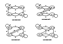
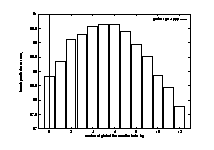
Figure 6, 7. 2bit Counter State Diagram Design
| Correlation Depth vs. Prediction Accuracy
(click each automaton for a full-sized figure)
From Figure 7 above, 5~6 global bits is the best choice when the branch prediction buffer is 8k bits. We use 5 bits in our comparison analysis since we used gcc here, and we expect fewer global bits should be used for floating point programs.
From Figure 8, we observe that the best choice is to use 3 global bits when the buffer is 8K bits.
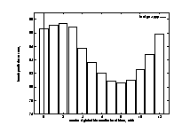
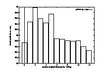
Figure 8-9. Local Scheme Correlation Depth vs. Prediction
Accuracy.
| Gshare Scheme Global Branch History Bit Adoption
vs Prediction Accuracy
From Figure 9 above, 2 global bits is best choice for 8kbit buffer case.
There are many variations in the design of selective prediction schemes. Two sub-predictors are chosen from different schemes. Given certain amount of prediction history buffer size, the three prediction history buffer may take different buffer spaces. McFarling used a gshare predictor and a bimodal predictor as the two sub-predictors. We use gselect and bimodal. Considering that it is more beneficial to have larger buffer size for gselect predictor, we use 2Kb buffer for the bimodal predictor, 4Kb buffer for the gselect predictor, and 2kb buffer for the selector. We use 3 global history bits for the gselect sub-predictor.
Providing the fast running speed of Shade, we can explore more schemes and run more programs. More importantly, we can trace much more instructions for each program. In our study, we traced most benchmark programs to the end. The regular size of a benchmark program is more than several hundred million and is getting larger. It may beyond the tracing and simulation capability of trace file based approaches to trace so many instructions. It is feasible for most trace file based approaches of trace and simulate at most several tens of million instructions. Since the branch behaviors of some programs will not show until program runs to the middle, our several hundred millions to several billions of instructions' tracing for each program is expected to provide more reliable result and more complete information about those benchmark programs.
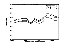
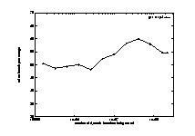
Figure 10, 11. Prediction Accuracies vs. Branch Instructions Traced
| Branch Taken Percentage vs. Branch Instruction Traced
To evaluate the performance of the seven different schemes, we first studied the branch behavior of the 21 benchmark programs that we use for this project. From this information, we are able to calculate the accuracy limit on the performance of a static predictor. Second, we give a comprehensive comparison of the seven schemes. Third we look at the effect of varying the buffer size on prediction accuracy for some dynamic schemes. Fourth, the effect of context switching on branch prediction is discussed. Finally, we look at an interesting benchmark program from SPECint95-beta.
| Program | Traced_Inst# | Dynamic_Branch# | Taken_Branch# | Taken_Branch% |
| gcc | 6186539354 | 1057556947 | 566093312 | 53.53 |
| ghost | 4057743776 | 690986805 | 339710533 | 49.16 |
| go | 9800796393 | 1078696639 | 504611777 | 46.78 |
| li+ | 7007645073 | 1000000000 | 551847194 | 55.18 |
| m88ksim+ | 7507989139 | 1000000000 | 479341651 | 47.93 |
| numi+ | 12355029197 | 1000000000 | 639221685 | 63.92 |
| perl+ | 8234202623 | 1000000000 | 474993437 | 47.50 |
| vortex+ | 7195515374 | 1000000000 | 425973672 | 42.60 |
Table 4. Branch behavior of benchmark programs from SPEC95int-beta
| Program | Traced_Inst# | Dynamic_Branch# | Taken_Branch# | Taken_Branch% |
| alivinn | 6792027933 | 480143481 | 469154917 | 97.71 |
| doduc | 1644410091 | 87092576 | 48388199 | 55.56 |
| ear | 14506557248 | 705032704 | 466983346 | 66.24 |
| fpppp | 8463667939 | 106307360 | 67686215 | 63.67 |
| hydro2d | 6627612755 | 680214394 | 515386882 | 75.77 |
| mdljdp2 | 4206065214 | 309377515 | 215543933 | 69.67 |
| mdljsp2 | 3011635408 | 338499291 | 195972810 | 57.89 |
| nasa7 | 11104431137 | 217326271 | 186014771 | 85.59 |
| ora | 2029511987 | 158386472 | 82174861 | 51.88 |
| su2cor | 8055850151 | 165611544 | 140751098 | 84.99 |
| swm256 | 9862718926 | 66039940 | 61056566 | 92.45 |
| tomcatv | 1261279753 | 31605162 | 30958962 | 97.96 |
| wave5 | 4331716191 | 286632343 | 194798779 | 67.96 |
Table 5. Branch behavior of benchmark programs from SPEC92fp
Conditional branch frequencies dramatically affect machine pipeline performance. Therefore, it is important to look at the percentage of conditional branches. Figure 12 lists the conditional branch frequencies for the 21 benchmark programs used in this study. The x-axis lists the 21 benchmark programs starting with the 8 integer programs. The y-axis shows the percentage of conditional branches. The integer programs show conditional branch frequencies of 8% to 17%, with numi having the lowest. As mentioned in the previous section, among all integer programs, numi is the only one written in Fortran and has the highest FP instruction percentage -- 10.2%. All the other integer programs are written in C. The FP programs have lower percentage of conditional branches then integer programs. They show frequencies between 1% to 11%. The average frequency for the 8 integer programs is about 14% and 5% for the 13 FP programs.
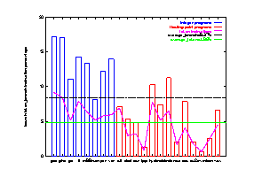
Figure 12 The Frequencies of Conditional Branches
In Figure 13, the frequencies of taken conditional branches are given. As in Figure 12, the x-axis lists the 21 benchmark programs, and the y-axis gives the percentage of taken conditional branches. The first 8 programs are integer programs. The horizontal dash line represents the average frequency for all the 21 programs. All of the 8 integer programs are below this average. numi is close to the average for the same reason in the earlier paragraph. Notice some of the FP programs have almost 100% taken frequency, such as alvinn and tomcatv. The average for the integer programs is about 50% and 75% for the FP programs. As you will see later, this frequency is directly related to prediction performance of all the predictors. Generally speaking, the higher the taken frequency, the higher the prediction accuracy. This is also shown in the earlier discussion of tracing instruction number. The prediction accuracy curves in Figure 10 have a similar shape as the branch taken percentage curve in Figure 11. FP programs are easier to predict than integer programs with low frequency of taken branches.
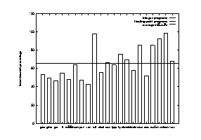
Figure 13 Percentage of conditional branches that are taken
The bias of a branch describes how strongly this branch tends to be taken or to be not taken. Profiling based Static predictors work well because that most of the dynamic branches executed are strongly biased. Figure 14 shows the bias over all integer benchmarks, over all FP benchmarks, and over all the 21 benchmarks. The average of each group is used. The x-axis shows for a particular branch the percentage of executed branches that are taken. Branches within 5% are grouped together as one group. The y-axis shows the percentage of branches that have a certain bias. The less frequent the number of branches in the middle, the better the performance of the perfect static predictor. We notice that the FP programs are more biased than the integer programs.
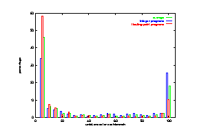
Figure 14 Branch bias, weighted by execution frequency.
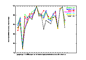 |
|---|


 |
| Figure 15 Seven schemes performance on the 21 benchmark programs |
| (Click the following hyper texts to have detailed views of the comparison.) |
| comparison of static, bimodal and common-correlation schemes |
| comparison of gshare, common-correlation, local and gselect schemes |
| comparison of gselect, local and selective schemes |
| comparison of gselect, local and common-correlation schemes |
| comparison of static, bimodal and selective schemes |
Figure 16 Seven schemes average prediction accuracy over the
21 benchmark programs
| Benchmarks | Schemes ordered by performance (from worst to best) | ||||||
|---|---|---|---|---|---|---|---|
| INT | static | bimodal | gshare | correlation | local | gselect | selective |
| 89.8% | 89.8% | 90.3% | 90.8% | 91.3% | 91.8% | 92.7% | |
| FP | static | bimodal | correlation | gshare | gselect | selective | local |
| 93.3% | 94.4% | 94.7% | 94.7% | 95.3% | 95.5% | 95.6% | |
| ALL | static | bimodal | gshare | correlation | local | gselect | selective |
| 92.0% | 92.6% | 93.0% | 93.2% | 93.9% | 93.9% | 94.4% | |
Table 6. Performance summary of the seven schemes
We observe the following:
The results are shown in Figure 17, with curves for the three dynamic schemes. The curve for the bimodal scheme goes flat when the number of 2-bit counters gets above about 5000. This agrees with results from previous research. Therefore, for the bimodal scheme, buffer size is not a limiting factor when it is more than 8K bits (4K 2-bit counters). The bimodal scheme behaves this way because in a typical run of program, 5000 different branches is considered to be large. Shown in Table 1 and Table 2, excluding gcc and vortex, all benchmarks studied have only between 1000 and 5000 static conditional branches. The common correlation scheme still has noticeable improvement with increased buffer size till 20K bits or 10K 2-bit counters. Even when the buffer size reaches 200K bits, the gselect scheme still shows significant improvement if the correlation depth is also increased accordingly.
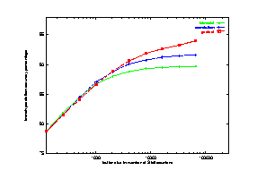
Figure 17 Effects of varying branch prediction buffer size
The results are shown in Figure 18, with curves for bimodal, correlation, and gselect. The three horizontal lines in the figure show the prediction accuracies for each scheme in the case of no context switch. For all three schemes, we observe that the effect of context switches on prediction rate decreases as the number of instructions between context switches gets larger. We see very little effect after the number of instructions is over 1 million.
Since the increased speed in CPUs, the number of instructions between context switches is getting larger. For a 50-MIPs machine, it is about 3 million instructions assuming the commonly used 16 context switches per second on a UNIX system. Therefore, context switching has little effect on branch prediction accuracy. However, threads and multiprocessing are increasing in importance. The number of instructions between context switches for these lightweight processes sometimes is much shorter than conventional context switches. For this reason, the effect of context switches should not be overlooked.
We also notice that for less complicated schemes such as bimodal, the effect of context switches is not as evident as for some more complicated schemes such as gselect. This indicates that complicated schemes need longer time to warm up than simple schemes.
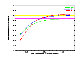
Figure 18 Effects of context switching on prediction accuracy
go is a special version of the "Go" program, "The Many Faces of Go", developed for use as a part of the SPEC benchmark suite. As described in the description file with the benchmark, go is an artificial intelligent game program. It is a computation bound integer benchmark and uses a very small amount of FP only during initialization to set up an array of scaled integers. It uses almost no divides, and few multiplies. Most data is stored in single dimensioned arrays specifically to avoid multiplies. This program has been extensively optimized using gprof to tune for maximum performance. Some inner loops have been unrolled in C. It features many small loops and lots of control flow -- if-then-else. This feature of go causes all the branch prediction schemes which take advantage of long looping structures to perform poorly. Does this say that complicated compiler optimization will change the program branch behavior and the prediction accuracy?
Figure 19 shows the bias of go with comparison to gcc and the average for the 8 integer programs. The curves for both gcc and the integer average show clear U-shape. However, the curve for go is quite flat. There are about same number of branches for each 5% interval of un-takenness. This distribution of branches causes various predictors to perform poorly. This result also indicates that the branch behavior is the most important parameter in determining the prediction accuracy of each scheme.
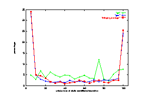
Figure 19 Profiling information for go
We look at the effect of increasing buffer size on prediction accuracy using go as the testing benchmark. For this part of the study, we used the gselect scheme. We varied the branch prediction buffer from 256 bytes to 64K bytes. For each buffer size, the history depth also need to be varied. Without increasing the correlation depth, increasing buffer size does not gain much improvement.
Figure 20 shows the results from this study. The x-axis shows the number of global history bits used (history depth). The y-axis shows the prediction accuracies. There is a curve associated with each buffer size. For each buffer size, there is one with the best prediction rate. We use another curve to connect all these points. For the 256 bytes buffer, the best prediction accuracy is about 76%. If 64K bytes buffer is in use, the best prediction accuracy can go up to about 88%, which has a 50% improvement in miss predict rate.
From the figure, we notice that for go, a highly correlated program, increasing the number of global history bits can help to improve the prediction accuracy. Since there are lots of if-then-else control structures in the benchmark, the direction of a branch usually depends on the outcome of others. Therefore, the predictor needs high correlation depth, which is larger than 15 indicated by the 64KB curve.
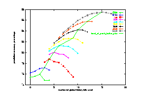
Figure 20 Effects of increasing branch prediction buffer size on go using gselect
The following findings may be of interest for future research
in branch prediction and new architecture design.