

Patrice Koehl
Department of Computer Science
Genome Center
Room 4319, Genome Center, GBSF
451 East Health Sciences Drive
University of California
Davis, CA 95616
Phone: (530) 754 5121
koehl@cs.ucdavis.edu

 |

| Patrice Koehl |
Modeling and Data Analysis in Life Sciences: 2017Project1: Simulation: The Logistic MapHandoutsSimulation: The Logistic Map
Word document (click to download) or PDF document (click to download) The Logistic MapLet us consider a population P that evolves under a discrete model, i.e. we follow the evolution of P(t) for time t that takes discrete values (we will assume t = 0, 1, 2,….). We consider a very simple model for this evolution. Let us assume that this population can take a maximum value Pmax. Instead of considering the value of the population P(t), we will instead compute X(t) = P(t)/Pmax. Note that X(t) takes values between 0 and 1. We consider a very simple model for the evolution of X(t): X(t) = R X(t-1) ( 1 - X(t-1) )Namely, the population at time t is is completely determined by its value one step prior. In this equation, R is a parameter between 0 and 4. Note that this model is intended to capture two effects:
This equation seems simple, but it generates unusual behaviors. You can learn more about it at: https://en.wikipedia.org/wiki/Logistic_map. We will study it as part of this project. Part ABelow is a small Matlab script that computes the evolution of X(t) over 100 values of t, with the initial value for X set to 0.5, and R set to 2.5:
R = 2.5;
Nval = 100;
time=0:1:Nval-1;

figure;
x=zeros(Nval,1);
x(1) = x0(i);
for j = 2:Nval
x(j) = R*x(j-1)*(1-x(j-1));
end
plot(time,x);
xlabel('Time')
ylabel('Population')
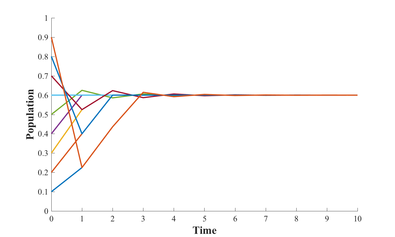
Starting from the code, you will generate 4 plots showing the evolution of X(t) for 4 different values of R, namely R= 0.5, R =2.0, R = 3.25, and R = 3.8. For each value of R, you will consider 9 different initial conditions, X = 0.1, 0.2, 0.3, 0.4, 0.5, 0.6, 0.7, 0.8, and 0.9, and show the corresponding evolutions of X(t) as a function of "time" on the same plot. Here is an example, for R = 2.5: 
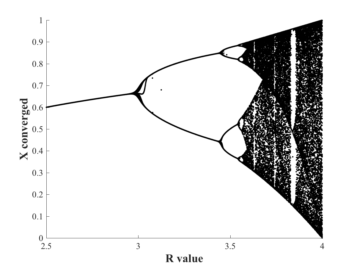
Do comment on the plots you observe! Part BIn part A, we have observed very different behaviors for the evolution of the population for different values of R. For some values of R, all trajectories seem to converge to that same value, while for other values of R, the population "converges" to different values for different initial values. Let us study this in more details. More specifically, for a large set of values of R between 2.0 and 4.0, you will store the end values of the trajectories of the population for a large set of initial conditions, and plot those values as a function of R. I am expecting a curve of the form: 
Make sure to explain what this curve means! Please provide both the source code of the program (s) you wrote, and a report describing the results. |
| Page last modified 15 June 2022 | http://www.cs.ucdavis.edu/~koehl/ |