AIX008: Introduction to Data Science: Summer 2022

Linear regression: building a model from data

The following hands-on exercises were designed to teach you step by step how to build linear models based on given data, assess and select the best of thse models based on training data, and finally to use this model to predict values on a test dataset. We use the "cebsus" dataset (available directly from Matlab), which contains information on the population of the USA from the time it was founded until 1990.

The question we would like to answer is can we predict the current population of the US in 2022?

The census data set

The census data is directly available from Matlab. It consists of two arrays, "cdate" that contains a set of dates from 1790 till 1990, and "pop" that contains the correspoinding population of the US, in millions. He is a small Matlab script that loads the data, and plots them using a scatter plot.

>> load census
>> figure
>> plot(cdate, pop, 'or', 'LineWidth',1.5)

And here is the plot: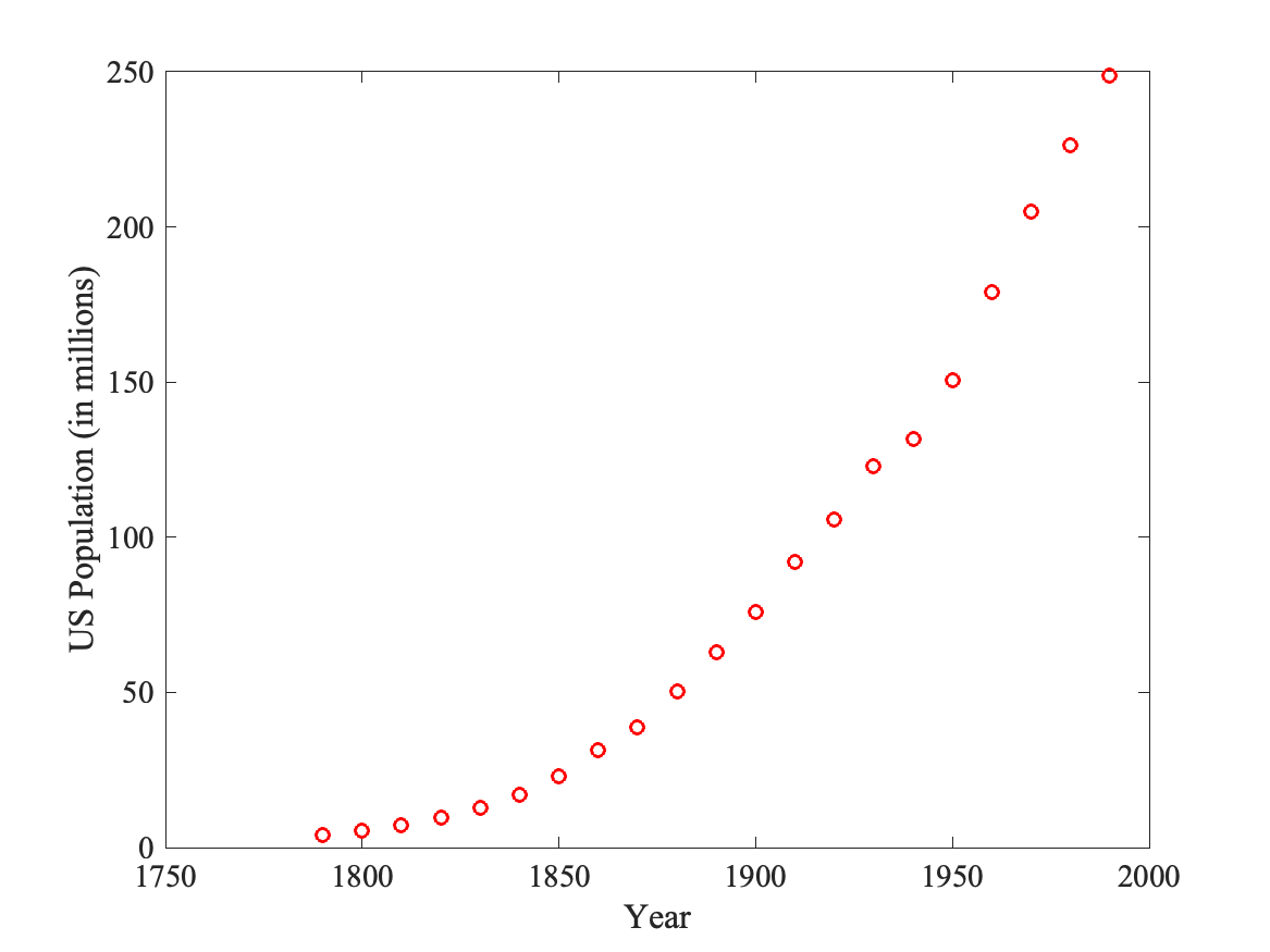

Prediction 1: A kNN model

Here is a small Matlab that implements a kNN predictor knn.m:

function val=knn(xtrain,ytrain,x,k)

% Compute array of distances between x and training set
dist=abs(xtrain-x);

% Sort array dist; keep indices 
[t,idx] = sort(dist);

% Reorder yvalues based on order idx
y=ytrain(idx);

% compute estimate of y
val = sum(y(1:k))/k;

return;

Using this function, fill up this simple table:

Question: all those predictions are poor. Can you explain why?

Prediction 2: a polynomial fit

Instead of just computing the value of the population for year 2022 using a kNN model, we use the census data to build a model y=f(date), and use this model to predict the population at the year 2022. We will use a polymomial model of order p (i.e. \( y = a_p x^p + a_{p-1} x^{p-1} + \ldots + a_1 x^1 + a_0 \) ), with p = 1 (fit with a line), p = 2 (fit with a second order polynomial), p = 3 (fit with a third order polynomial) and p = 4 (fourth order polynomial).

You will use the two Matlab functions "polyfit" and "polyval", as well as the "Basic Fitting" Tools in a figure.

Using these function, fill up this simple table:

Draw on the same plot the different fits obtained for polynomials of degree 1, 2, and 4. The predictions based on a linear fit are significantly better. Can you explain why?