AIX008: Introduction to Data Science: Summer 2022

Activity: Getting to know Matlab

With this lab, you will start becoming familiar with the Matlab environment and some of its facilities. You will learn:

• - How to perform basic arithmetic operations
• - How to assign values to variables
• - How to use control structures (do and if)
• - How to generate graphics

Exercise 1: Basic Arithmetic calculations within Matlab

Evaluate the following expressions by hand and use Matlab to check the answers:

1. \(1+2+3\)
2. \(\cos(\frac{\pi}{6})\)
3. \({3^{2}}^{2}\)
4. \(\log(e^{3})\) (lookup the functions exp and log)
5. \(\sin^2\left(\frac{\pi}{6}\right) + \cos^2\left(\frac{\pi}{6}\right)\)

Exercise 2: assign values to variables; basic operations on arrays

1. \(f = \cos(x)\sin(x)\)
   ans =
   0.4546 -0.3784 -0.1397
2. \(f = (\sin(x))^2\)
   ans =
   0.7081 0.8268 0.0199
3. \(f = \sin(x^2)\)
   ans =
   0.8415 -0.7568 0.4121
4. \(f = 7x^2 \sin \left(\frac{1}{7x^2}\right)\)
   ans =
   0.9966 0.9998 1.0000

Exercise 3: Control structures

We consider the famous Fibonacci sequence that was originally developed to characterize the population of rabbit. It is define as follows: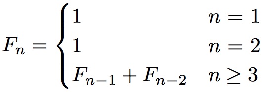

For example, starting with n = 1, we get: 1,1,2,3,5,8,13,21 ...

Write a Matlab script that computes F_n. Check it for n = 5, 10, and 20.

Exercise 4: Plotting

We want to create a graph of \(y=cos(4x)\) over \([0, \pi]\). To illustrate what happens when there are too few points in the x domain, let us first try a step size of \(\pi/10\).

• Which command gives the desired values for x?
  
  1. x = 0:pi:pi/10;
  2. x = 0:pi/10:pi;
  3. x = 0:1/10:pi;
• Which command gives the correct answer for y?
  
  1. y = cos(4x);
  2. y = cos4*x;
  3. y = cos(4*x);
• Plot your graph with the plot command
• Redo your plot, this time using the command
  >> x = linspace(0,pi)
  to define the x array. Which plot looks more like the plot of a cosine curve?

Exercise 5: Errors in programs

The following Matlab programs contain some elementary programming mistakes. Find the mistake and suggest a solution to each or them.

• Program 1:
  

  function d=pol2(h)
  d=0;
  i=0;
  while i < h
  d=d+1;
  end
  

  
  
• Program 2:
  

  function diff =pol3(arr)
  for i=1:length(arr)
    diff(i)=arr(i)-arr(i+1);
  end
  

  
  
• Program 3:
  

  r=input('Please enter a number: ');
  if r=0
  fprintf('The number is zero');
  else
  fprintf('The number is negative');
  

  
  

Exercise 6: graphing

Biorhythms were very popular in the 1960s. They are based on the notion that three sinusoidal cycles influence our lives. The physical cycle has a period of 23 days, the emotional cycle has a period of 28 days, and the intellectual cycles has a period of 33 days. For an individual, the cycles are initialized at birth. The figure below shows my biorhythm, which begins on October 26, 1961, plotted for an eight-week period centered around Wednesday, June 29, 2022.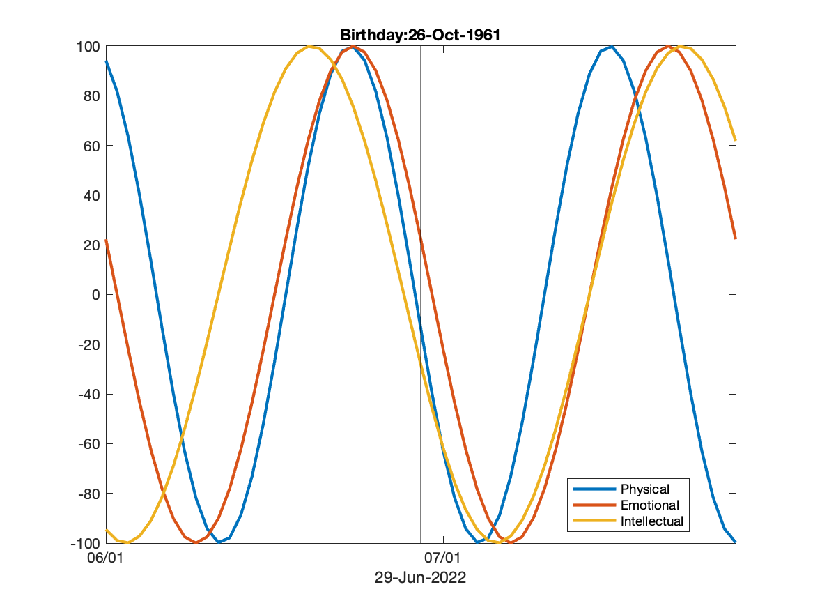

The following code segment is part of a program that plots a biorhythm for an eight-week period centered on the date June 29, 2022

t0 = datenum('Oct. 26, 1961');
t1 = datenum('June 29, 2022');
t = (t1-28):1:(t1+28);
y1 = 100*sin(2*pi*(t-t0)/23);
y2 = 100*sin(2*pi*(t-t0)/28);
y3 = 100*sin(2*pi*(t-t0)/33);

plot(t,y1,'LineWidth',2);
hold on
plot(t,y2,'LineWidth',2);
plot(t,y3,'LineWidth',2);

• Complete the program above, using your own birthday, and the line, datetick, title, datestr, legend, and xlabel functions. Your program should produce something like the figure above.
• The three rhythms are periodic functions, with periods 23, 28, and 33 days. There will be a day in your life when all three rhythms will be zero again ("resetting" the rhythms): it will occur 23*28*33 days after your birth, i.e. on day 21252, i.e. when you will be 58 years old! Can you find which day this will be?
• In between your birthdate and that day, is there a day where all your 3 biorhythms will be maximum? The answer is no... but can you find a "near perfect" day, i.e. a day where the three biorhythms will be close to 1?
  Hint: Consider finding the maximum of the sum of the three functions y1, y2, and y3