AIX008: Introduction to Data Science: Summer 2022

Application of kNN for classification

The following hands-on exercises were designed to teach you step by step how to build k-NN models based on given data, assess and select the best of thse models based on training data, and finally to use this model to classify test dataset. We use the "Wisconsin breast cancer" dataset (available locally at breast_cancer.csv, which contains information on 569 patients suspected of having breast cancer. For each patient, a biopsy was performed. The actual diagnosis from that biopsy is known (i.e. either the biopsy is "benign" or "malignant". In addition, an analysis of the image of cells from the breast tissue was performed. Ten different features were measured:

• radius (mean of distances from center to points on the perimeter)
• texture (standard deviation of gray-scale values)
• perimeter
• area
• smoothness (local variation in radius lengths)
• compactness (perimeter^2 / area - 1.0)
• concavity (severity of concave portions of the contour)
• concave points (number of concave portions of the contour)
• symmetry
• fractal dimension ("coastline approximation" - 1)

For each feature, three values are reported, the mean over all cells in the image, the standard error, and the "worst" value, i.e. the value that differs the most from the mean.

The question we would like to answer is:

Can we classify the biopsy based on the features of the cells in the image?

The breast cancer data set

We first examine the relationships between the features and diagnosis separately. For simplicity, we replace the "B" for benign with 0, and the "M" for malignant with 1. Here is a small Matlab script that reads in the dataset, and illustrates those relationships as scatter plots for three features, Radius, Area, and Fractal dimension. Here is the MATLAB script: read_cancer.m

>> cancer=readtable("breast_cancer.csv");
>> cancer=rmmissing(cancer);
>> figure
>> subplot(1,3,1)
>> subplot(1,3,1)
>> plot(cancer.Radius,cancer.Diagnosis,'or')
>> xlabel('Radius')
>> ylabel('Diagnosis (0:Begnin, 1:Malignant')
>> subplot(1,3,2)
>> plot(cancer.Area,cancer.Diagnosis,'or')
>> xlabel('Area')
>> ylabel('Diagnosis (0:Begnin, 1:Malignant')
>> subplot(1,3,3)
>> plot(cancer.Fractal,cancer.Diagnosis,'or')
>> ylabel('Diagnosis (0:Begnin, 1:Malignant')
>> xlabel('Fractal')

And here are the plots: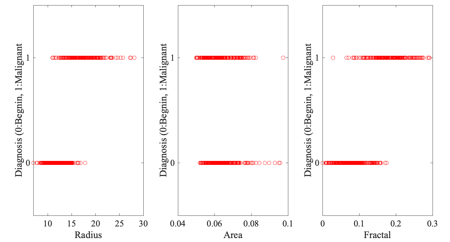

None of the features by itself correlate well with diagnosis, with Radius doing a little better. We will then build first kNN models based on Radius alone.

A kNN model to predict cancer diagnosis based on Radii of the cells

Our tast is to build kNN models from Radius alone, choose the best of these models based on a training set, and finally use this model on a test set. To do this, I have divided the breast cancer dataset into three sets:

• A DATA set: cancer_data.csv
• A Training set: cancer_training.csv
• A Test set: cancer_test.csv

>> data=readtable("cancer_data.csv");
>> train=readtable("cancer_training.csv");
>> test=readtable("cancer_test.csv");
>> data.Diagnosis=categorical(data.Diagnosis); % Transform diagnosis into categorical variable
>> data.Diagnosis=renamecats(data.Diagnosis,{'B','M'},{'0','1'}); Recast "B" to "0" and "M" to "1"
>> data.Diagnosis=str2double(string(data.Diagnosis)); convert string to number
>> train.Diagnosis=categorical(train.Diagnosis);
>> train.Diagnosis=renamecats(train.Diagnosis,{'B','M'},{'0','1'});
>> train.Diagnosis=str2double(string(train.Diagnosis));
>> test.Diagnosis=categorical(test.Diagnosis);
>> test.Diagnosis=renamecats(test.Diagnosis,{'B','M'},{'0','1'});
>> test.Diagnosis=str2double(string(test.Diagnosis));
>> data_val=[data.Radius data.Diagnosis];
>> train_val=[train.Radius train.Diagnosis];
>> test_val=[test.Radius test.Diagnosis];
>> figure
>> plot(data_val(:,1),data_val(:,2),'ok','LineWidth',0.5);
>> hold on
>> plot(train_val(:,1),train_val(:,2),'ob','LineWidth',1.5);
>> plot(test_val(:,1),test_val(:,2),'or','LineWidth',1.5);
>> xlabel('Radius')
>> ylabel('Diagnosis (0:Begnin, 1:Malignant')
>> ylabel('Diagnosis (0:Benign, 1:Malignant')
>> legend('Data','Train','Test')

And here is the plot: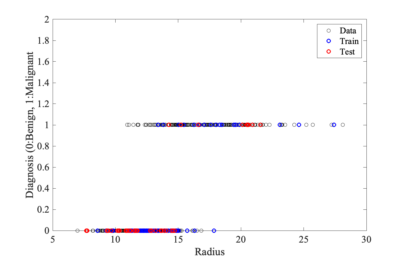

The following Matlab script build a 1-NN model from the Data set and uses the training set to evaluate it using the number of correct prediction (in percentage); It also plots the actual diagnostic and predicted diagnostic for the training set. Here is the MATLAB script: cancer_1NN_radius.m

>> ntrain=max(size(train_val)); % number of training data
>> rmse=0;                      % Initialize RMSE to 0
>> for i = 1:ntrain             % For each training point
val = train_val(i,1);           % Radius value for this point
dist=abs(data_val(:,1)-val);    % Computes distance to all points in DATA
[t,idx]=sort(dist);             % Sort these distances
y=data_val(idx,2);              % Order the Diagnosis value in DATA set accordingly
y_predict(i) = y(1);            % This is a 1-NN: pick the first value
if train_val(i,2) == y(1)       % check if predicted is correct
rmse = rmse + 1;
end
end                             % end loop
>> rmse = 100*rmse/ntrain;    % Compute percent correct
>> figure
>> plot(train_val(:,2),y_predict,'or','LineWidth',1.5);
>> xlabel('Actual diagnostic')
>> ylabel('Predicted diagnostic')
>> title("RMSE = " + rmse);

We find that the 1-NN is "reasonable", with a prediction correct 78.75% of the time on the training set.

After adapting this script, you will:

• Repeat this analysis over the training set, build k-NN models for k = 2, 3, ...., 10
• Plot the corresponding prediction rate values against k. Pick the best k, k_best
• Build a k-best-NN model on the DATA set, and test it on the TEST set. What is the corresponding prediction rate?

A kNN model to predict diagnostic based on all image features

The analysis you have performed above was based on Radius only. Repeat the whole analysis, using now all features. I provide the corresponding script for the 1-NN: cancer_1NN_all.m

>> data_all = [data.Radius data.Texture data.Perimeter data.Area data.Smoothness ...
data.Compactness data.Concavity data.ConcavePoints data.Symmetry data.Fractal data.Diagnosis];
>> train_all = [train.Radius train.Texture train.Perimeter train.Area train.Smoothness ...
train.Compactness train.Concavity train.ConcavePoints train.Symmetry train.Fractal train.Diagnosis];
>> ntrain=max(size(train_all));
>> ndata=max(size(data_all));
>> rmse=0;
>> for i = 1:ntrain
val=train_all(i,1:10);
for j = 1:ndata
dist(j) = norm(data_all(j,1:10)-val);
end
[t,idx]=sort(dist);
y=data_all(idx,11);
y_predict(i) = y(1);
if train_all(i,11) == y(1)       % check if predicted is correct
rmse = rmse + 1;
end
end
>> rmse=100*rmse/ntrain;
>> figure
>> plot(train_all(:,11),y_predict,'or','LineWidth',1.5);
>> xlabel('Actual diagnostic')
>> ylabel('Predicted diagnostic')
>> title("RMSE = " + rmse);

This shows that the 1-NN based on ALL data is "reasonable" and better than the 1-NN based on Radius only, with a RMSE of 86.25 %.

After adapting this script, you will:

• Repeat this analysis over the training set, build k-NN models for k = 2, 3, ...., 10
• Plot the corresponding prediction rate values values against k. Pick the best k, k_best
• Build a k-best-NN model on the DATA set, and test it on the TEST set. What is the corresponding prediction rate?